Heuristics in Optimisation

Another fortnight, and another 10 presentations on research in STOR-i. The current phases of the MRes program is starting to introduce us to the different research areas that we may be able to choose our PhD topic in. There was also a fantastic performance by the Lancaster University Korfball team at BUCS North Regional competition, which you can see for yourself on the Lancaster University Korfball Facebook page.

Korfball brilliance aside, one of the research topics we’ve seen was from Dr Ahmed Kheiri (a lecturer in the Lancaster University Management School) called “Heuristic methods in hard computational problems”. This is an area I’ve previously had some experience in, so I thought it would be a good idea to dive a bit deeper into this.

An overview of optimisation

Optimisation is the general area of maths of finding the highest or lowest solution to a problem, often given some constraints. A very simple example of this is a furniture maker, who has a certain amount of wood, and needs to decide how many chairs or tables to make to maximise profit, given the limits to the amount of wood each requires, and the amount of time they have to work on the problem. This problem could be formulated as:

Maximise (profit per chair x number of chairs made) + (profit per table x number of tables made)

subject to:

(wood used per chair x number of chairs made) + (wood used per table x number of tables made) ≤ Total wood available

and

(time taken to make a chair x number of chairs made) + (time taken to make a table x number of tables made) ≤ How much time they have

and finally

Number of chairs and number of tables are integers (i.e. you can’t make half a table/chair)

I’ll also use this problem to introduce some terminology:

• The objective function is the mathematical expression you are trying to maximise/minimise. In this example, it is the first expression containing the profits of the chairs and tables.
• The constraints are the mathematical expressions which you have to abide by to solve the problem. In our example, these are the expressions saying you can’t use more wood or time than you have.
• The decision variables (often just called the variables) are the values that you can change to optimise the objective function. This this example, the variables are the number of tables and chairs to make.
• If some given values of the variables satisfy the constraints, this is called a feasible solution.
• The set of all feasible solutions (i.e. every possible combination of tables and chairs that we could make with our wood and time) is called the solution space.

This is a very simple optimisation problem, and you could probably find solution to it quite quickly (either directly, or through some established algorithms). However, these sorts of problems can quickly get out of hand. What if you actually have more products than you can make from your wood? What if the first few chairs sell for a higher cost than the next few? What if you have to sell chairs and tables as a set?
The more complicated the problem is, the (computationally) harder it will be to solve exactly. However, if you’re willing to cheat a bit, there are some methods that can help.

Heuristics

A heuristic is really any optimisation technique/algorithm for finding a good or approximate solution very quickly. It can be something as simple as the following:

1. Randomly pick any feasible solution to the problem, and take it as the current best solution.
2. Randomly pick any new feasible solution to the problem.
3. If the new solution is better than your current best solution, replace your current best solution with the new one
4. Repeat steps 2 and 3 until you are satisfied that you either have a good enough solution, or you are sick of running the algorithm.

There are two points about the above algorithm. Firstly, it will (the longer you do it) find a better solution; but secondly, there’s no guarantee that it’ll get there any time soon, or any guarantee that it’ll get close to the true best solution. This is because it’s just randomly jumping all over the solution space. It’s not actually looking for a good solution – it’s just stumbling around, hoping to find one.

A better heuristic will often try to move in the “direction” of better solutions. A classic example of this is the gradient descent method:

1. Pick a point in the solution space. Call this your current best solution
2. Calculate the gradient of the solution space at your current best solution
3. Move a step in the solution space in the direction of the gradient. Call this new point your current best solution.
4. Repeat until the gradient equals (or is suitably close to) 0.

The basic idea is to imagine putting a ball on the surface of the solution space, and letting it roll down, it will eventually settle in the lowest point. A very good gif of this is shown below (taken from the MI-Academy website)

Think of your solution space as the surface of a table. Gradient descent is kind of like putting a ball table and simply letting the ball roll down to find the lowest point.

It’s quite clear from the above gif that this is a much better heuristic. However, there are still situations in where this doesn’t work to well. Imagine we have the following objective function:

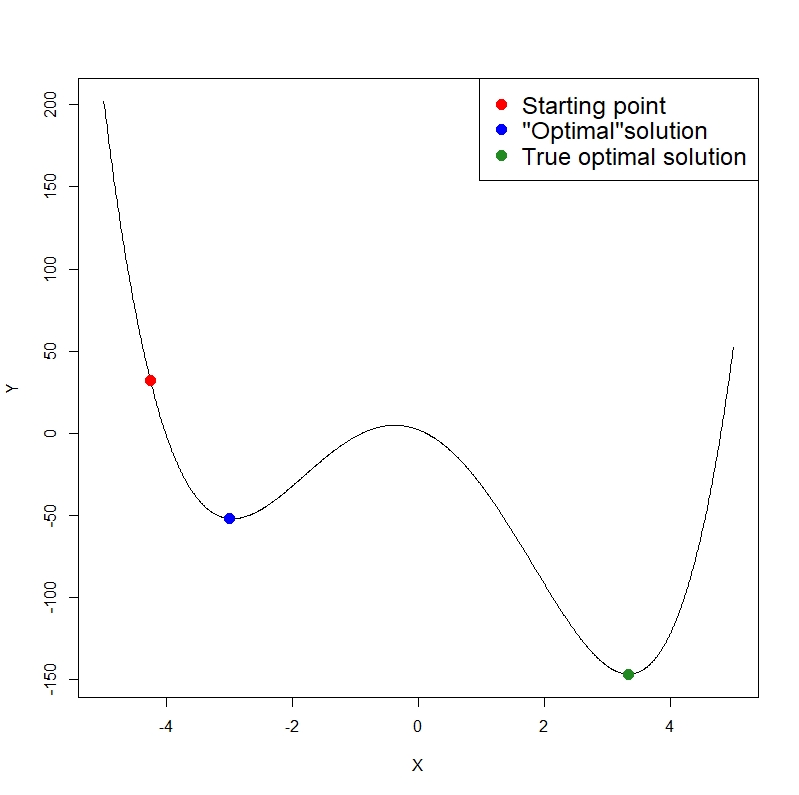
If you can imagine placing a ball at the red point, it will roll down and settle at the “minimum” at the blue point. While this is the minimum for this bit of the solution space (we call this a local minimum), it completely misses the true minimum (or global minimum) at the green point.

In general, the more complicated the function, the more sophisticated the heuristics needed to find a good solution.

Optimal wind turbine placement

Moving back to the presentation by Dr Kheiri, we look at the problem of optimal wind turbine placement. To quote the presentation:

The problem involves finding the optimal positions of wind turbines in a 2
dimensional plane, such that the cost of energy is minimised taking into
account several factors such as wind speed, turbines features, wake effects and
existence of obstacles

This problem will have many local minima, and so gradient decent will probably fail if we tried to use it.

The way this was solved in the paper was to use a genetic algorithm. This is a heuristic which tries to mimic natural selection in animal populations. The idea is that you generate a population of solutions, then you pick pairs of solutions from this population and from them “breed” new solutions, which have features from both of their “parent solutions”. The new solutions are then evaluated and the strongest (i.e. the best) survive, and the others are discard. This new solutions are then used to breed more solutions, and the process is repeated until you decide to stop.

Applying this to our wind turbine problem, we first set up our data as a binary vector of 1s and 0s. We do this by diving the plane into a 2-dimensional grid, with at most 1 turbine in each cell. Therefore, each cell is now associated with a binary variable, which takes the value of 1 if there is a turbine in it, and 0 otherwise. The decision then is which cells to but a wind turbine in (i.e. assign to a value of 1) and which to leave. From our matrix of 1s and 0s, we simply organise it into one long vector of turbine locations (mainly for computationaly simplicity), as shown in the gif below (in this example, every cell is a 1, but in truth, they will be a mix of 1s and 0s).

Once have set this up, we can start our genetic algorithm. First, we then generate a bunch of solutions, pair them off, and start breeding new solutions from these pairs. The breeding has two aspects:

1. Crossover: This is taking some parts of both the mother and father solution, and incorporating these into the child solution
2. Mutation: Randomly changing some aspect of the child solution. This helps the algorithm avoid getting stuck in a local minimum.

The breeding is shown below (again, in this example, the mother and father are the same, but in reality, they will be different).

We then see how good all these child solutions are, and keep the best ones. From these, we breed more new solutions, keep the best, and so on. We keep doing this until we are satisfied we have a good solution.

Hyper-heuristics

By this point, you probably are starting to realise the many different types of heuristic you could use to solve an optimisation problem. However, this leads to an obvious question – how do you chose which one? Some will converge quite quickly (e.g. gradient descent) whereas some will be more robust against local minima (genetic algorithms). In general there is no such right answer.

However, for a given problem, it is possible to apply a number of different heuristics, and then use a hyper-heuristic (also called a meta-heuristic). The way it works is to start with a number of low-level heuristics. You then run them over the problem, and (when you would normally iterate you one chosen heuristic) you switch between heuristics. This could be as simple as changing between the breeding rules in genetic algorithms, or switch search methods altogether. Ideally, you would also keep track of how each heuristic is doing as you go, and use this information to help chose your next heuristic.

In summary

• Heuristics are methods to help you quickly find a “good” solution to an optimisation problem (but not necessarily the best “solution”)
• They can range from pretty much useless (random search), to quick but error-prone (gradient descent) to slow and robust (genetic algorithm)
• There’s no “one best” heuristic. Each hang strengths and weaknesses which suit different problems.
• Moving forward, one of the big developments will be the use of hyper-heuristics, to determine which is the best method to use for your problem.