XVII Hydrogen atom
The Hydrogen atom consists of an electron of mass and negative charge , and a nucleus, which is a proton of positive charge and mass . The total Hamiltonian of electron and proton is given by
| (332) |
where the potential energy is the Coulomb energy of the two attracting charges.
XVII.1 Separation of relative and centre-of-mass motion
We introduce the centre-of-mass coordinate and the relative coordinate . The Hamiltonian then takes the form
| (333) |
where is the total momentum, is the total mass, is the momentum of the relative motion, and is the reduced mass. Since , . We consider the atom at rest, . Then we have to solve the Schrödinger equation
| (334) |
XVII.2 Separation of radial and angular motion
The Coulomb potential only depends on and hence is a central potential. Therefore, the solutions of the Schrödinger equation are of the form
| (335) |
where are the spherical harmonics of Eq. (244).
XVII.3 Radial motion
The radial equation (243) now takes the form
| (336) |
We introduce the rescaled radial coordinate
| (337) |
and the new parameter
| (338) |
and look for solutions . Equation (336) then takes the form
| (339) |
This equation is known as Kummer’s differential equation. For integer values , the solutions are given by , where are the Laguerre polynomials:
| (340) |
XVII.4 Energies
Since the energy levels of the Hydrogen atom only depend on the principal quantum number but not on or :
| (341) |
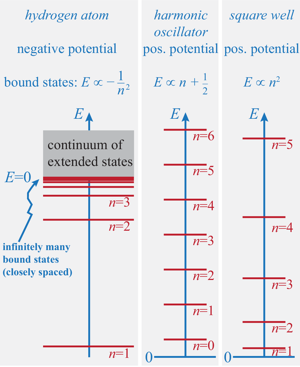
The energies can also be written as where Ry eV is the so-called Rydberg energy and m is called the Bohr radius.
The lowest energy level has energy eV. For energy , the electrons are not bound to the nucleus. Hence the Rydberg energy is the amount of energy required to release the electron from the nucleus (this process is called ionisation).
XVII.5 Spectral lines
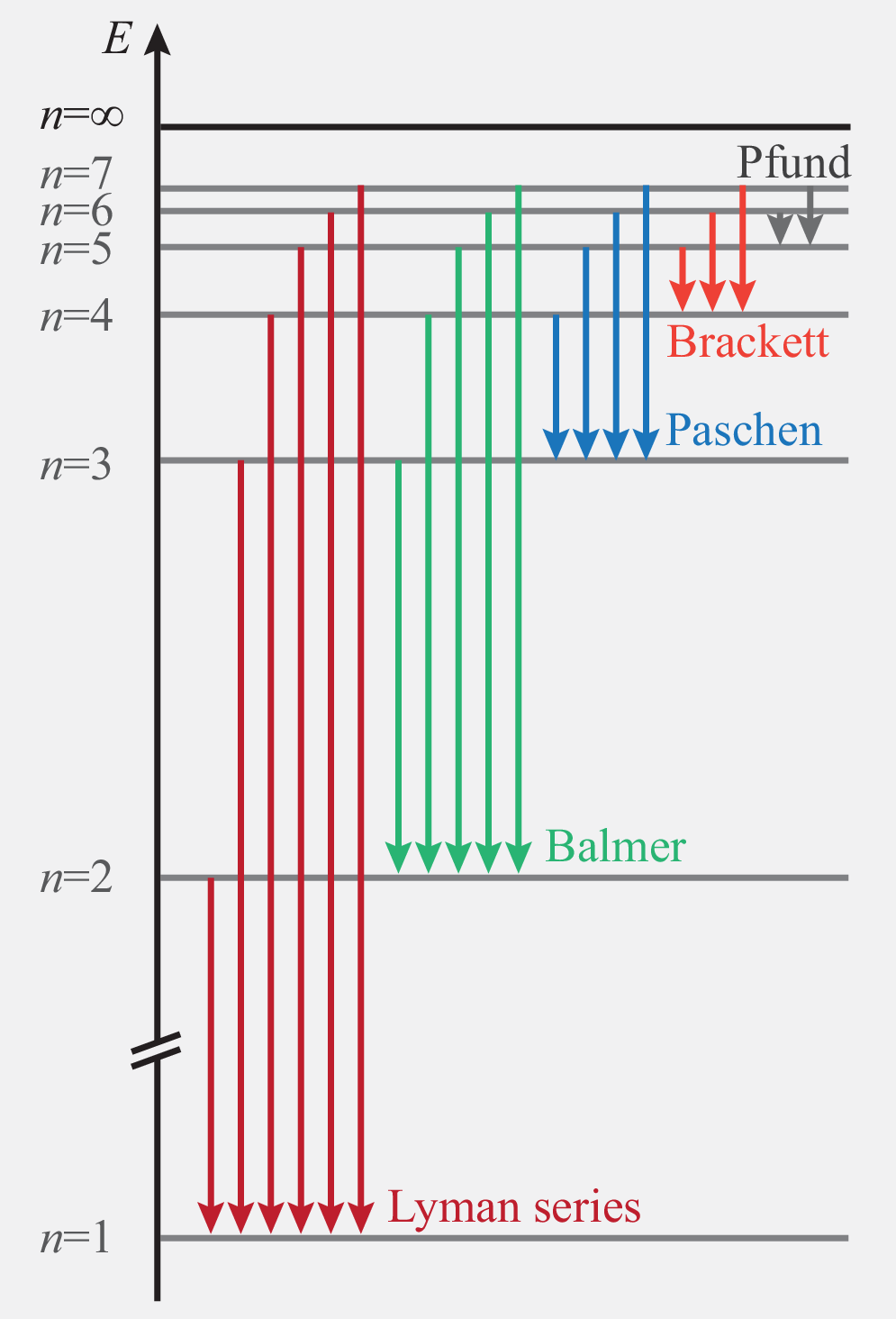
The electron can change from one energy level to another level if it absorbs or emits a photon which carries the right amount of energy . This gives rise to discrete spectral lines. The most important lines are grouped into series, such as the Lyman series (), the Balmer series (), and the Paschen series ().
XVII.6 Degeneracy
For each the allowed values of are , and for each there are allowed values of . Hence, the degeneracy of each energy level is . Later we will learn that the electron has an intrinsic degree of freedom called spin so that the degeneracy of each energy level is really . On the other hand we neglected small perturbations which lift the degeneracy and result in a fine structure of the energy levels. They will be discussed in the third year module PHYS321, Atomic & Nuclear Physics.
XVII.7 Atomic orbitals
The wavefunctions
| (342) |
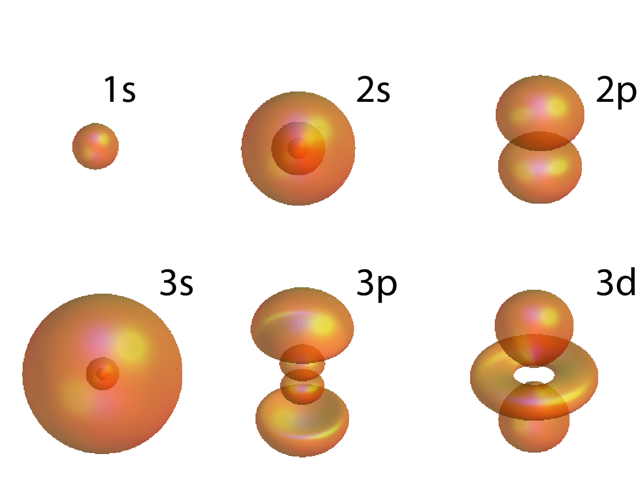
of the hydrogen atom are also called atomic orbitals. The azimuthal quantum number is denoted by a symbol s for , p for , d for , and f for . These symbols are then preceded by the principal wavenumber , so that orbitals are denoted by 1s, 2s, 2p, 3s, 3p, 3d etc.
XVII.7.1 Ground state
The ground state is associated with the spherically symmetric orbital 1s with energy Ry,
| (343) |
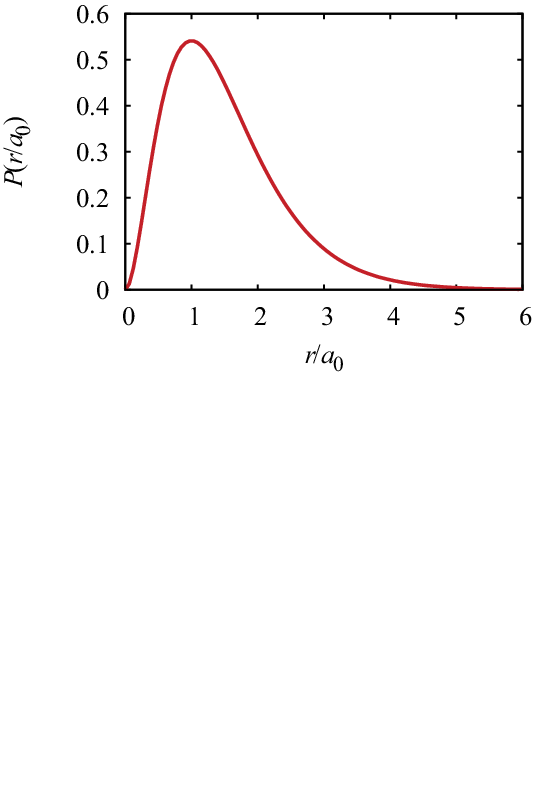
The probability density to find the particle in a shell of width at distance is given by
| (344) |
This probability density is maximal at .
XVII.7.2 First excited state
The first excited state has energy and is fourfold degenerate. It consists of the one 2s orbital and three 2p orbitals. The 2s orbital (, ) is spherical symmetric,
| (345) |
The 2p orbitals are not spherical symmetric,
| (346) | |||||
| (347) |
XVII.7.3 Second excited state
The second excited state has energy and is nine-fold degenerate. It consists of one 3s orbital, three 3p orbitals and five 3d orbitals.
XVII.7.4 Pictures of atomic orbitals
Figure 11 depicts surfaces of constant probability density for the lowest orbitals of the hydrogen atom.
XVII.8 Application: The Zeeman effect
We consider the hydrogen atom in a constant magnetic field , which points into the direction. The total magnetic moment of the electron is [see Eqs. (274) and (280)]
| (348) |
The interaction energy of the magnetic moment with the magnetic field is
| (349) |
The total Hamiltonian is given by
| (350) |
The Schrödinger equation is solved by
| (351) | |||||
| (352) |
where are the orbital wavefunctions of the hydrogen atom. These functions are eigenfunctions of :
| (353) |
where is the Bohr magneton. However, the degeneracy of the eigenvalues is now lifted,
| (354) |
The splitting of the levels depends linearly on the strength of the magnetic field.
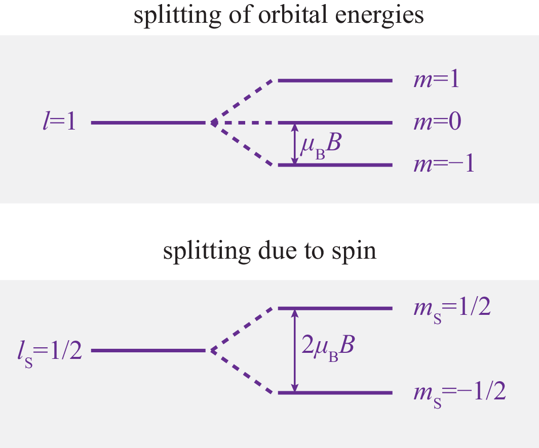
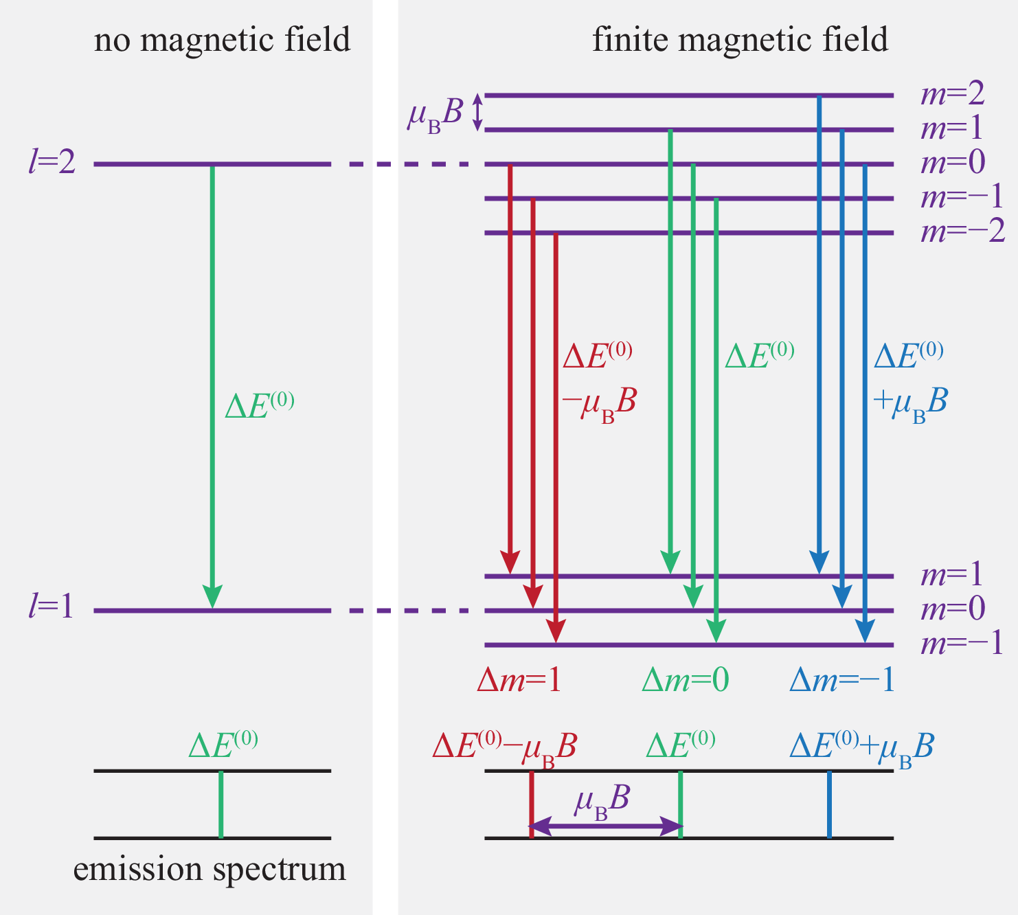
The splitting of the orbital energies can be observed in the spectral lines of the hydrogen atom. This is called the Zeeman effect. The observable spectral lines is restricted by selection rules: can only change by , , or , because of properties of the emitted photons. Since cannot change, the spin splitting is not observed in the normal Zeeman effect.