Problems with Police Cars and Pricing
26th February 2016
In the last week, STOR-i has put on two Probelm Solving Days. These are opportunities for all of the STOR-i students
to spend a day on a problem faced by a business or industry. The problems can be quite varied in topic and we have had
various companies come to ask for some ideas on how to tackle the issue. As it is only a few hours long, we are rarely
expected to have solved the problem and it is more about considering methods and approaches that could pave the way
towards a solution. The guest companies have ranged from EDF to West Yorkshire Police Service. Towards the end of the
day, the groups come back together to present their ideas. It is important that when presenting the ideas, they are
accessible to the people we are resenting to
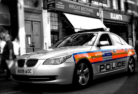
Last Friday, it was West Yorkshire Police who came with their
problem of how to decide how many Police cars, and of what
type, should their Force have as part of their fleet. The fleet managers explained to us that a large proportion of the
time, Police cars are parked up at the yard. In these times of austerity, the Police want to make sure that they make the
most of any assets they have, and so they were wondering how many cars they actually needed. The data given to us
included the maximum number of cars out at any time per day over three months.
After we had been given the problem, we split into groups and began to think of solutions. I would like to describe some
of these. The majority of the groups went about this problem in terms of how many marked cars would the Police need to cover a
day that occurred once every $N$ years. This is when extreme value theory (as discussed in Tails,
Droughts and Extremes) come into play. As the data is the maximum values every day, the approximation was made that
each day was independent and identically distributed. After this, the Generalised Extreme Value distribution was fitted
and estimates for the number of cars needed to cover a day that occurred with probability $p$. These showed that, even for
days that occur once every 100 years, the 95% confidence intervals for the number of cars was well below the current number
of cars! This suggests that the West Yorkshire Police could reduce the fleet size of marked cars by quite a lot.
The approximation made was pointed out by Professor Jon Tawn, and he said
he was surprised that it would hold. That at least made me feel a little better about not using it in our group.
Another group took quite a different approach indeed. They applied queueing theory to the situation. For this, they used the
number of incidents a day and as a Poisson process with a certain probability of the incident being classed as an emergency,
priority or standard. Each of the classes has a different expected number of cars going out to an incident and so would take
up a certain number of “servers”. The idea was to use an infinite server queue, which will always have enough cars to cope
with the demand, and to compare this with a system with $C$ cars. Once the number of cars $C$ was big enough to be a good
approximation to the infinite server queue, this $C$ was taken as the number of cars required by the Police. This method
also suggested that the number of cars could be reduced considerably. More surprisingly though, it actually produced a number
not dissimilar to that of the Extreme value theory method.
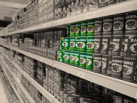
One the Problem solving this week (on Wednesday), the Chief Executive of a company called VYPR
came in to set us a problem of how to set prices at a supermarket with a new product. This is a big problem for supermarkets,
as getting the price too low will mean that it sells too much at the expense of other similar products in the same store. Set
the price too high and it simply won’t sell. VYPR are a company that sends out “steers” (or quick surveys) to people via their
smart phones. These steers could be used to gather information about what the public feel they would be willing to pay for a
new product.
Our task was to design such a steer. The steer could have at most 10 questions, and had to be easy to set up for a
non-statistician. The inputs for the steer must be straightforward and the outputs must be easy to interpret. However, we had
to take into account the behaviour of the person who was completing the steer.
For some reason, the solutions that the groups came up with were less varied than on the previous Problem Solving Day.
The general conclusion was that Bayesian Statistics was the right approach. Generally speaking, everyone decided that
the optimal price should be given a Beta prior. That is, if the supermarket set minimum and maximum prices, $P_\min$
and $P_\max$, the belief about the best price, $P$, is represented by the probability distribution with density
$$\pi(P) \propto \left(\frac{P-P_\min}{P_\max-P_\min}\right)^{a-1}\left(1-\frac{P-P_\min}{P_\max-P_\min}\right)^{b-1}$$
for some $a,b>0$ and $P$ between $P_\min$ and $P_\max$. The values of $a$ and $b$ give quite a range of distributions.
Our group thought it sensible to set the mean of the prior to be the average price for similar products already on the
market. Combining this with how important the supermarket thought that price was, we could in principle find out what the
correct values of $a$ and $b$ were.
The idea of Bayesian statistics is to combine this with the data from the surveys, $x$, via a likelihood function $f(x|P)$,
to produce a new probability distribution of the updated beliefs about $P$ called the posterior $\pi(P|x)$:
$$\pi(P|x) \propto \pi(P)f(x|P)$$
It was how the data was collected that was varied amongst
the groups. Our group settled on splitting the range between $P_\min$ and $P_\max$ into intervals, asking whether or not
someone would pay a price in an interval multiple times to discover which interval they were prepared to pay. The interval
number was taken as the random variable from a Binomial distribution. Whilst this is strictly not how a Binomial distribution
behaves, it does make the maths easy. To prevent the consumer guessing the system, the order of interval used was random. At
the end, the posterior distribution for $P$ would be given back to the supermarket, and they could then decide what the best
price is.
Other groups came up with different methods which mainly did not use the binomial distribution. This was probably more correct,
and it is only really through problem solving days that one can see other ideas, which is one of the best parts of a Problem
Solving day.