
Often times whether we are thinking about individuals or as a business, we may have to make decisions while considering future events and decision times. An example could be whether we decide to spend money today, or save money for tomorrow. This can be modelled by what is known as a Markov Decision Process (MDP). Here, we have a model with our current state and at certain time periods, we have decisions to make which is associated with probability of transitions to another state.
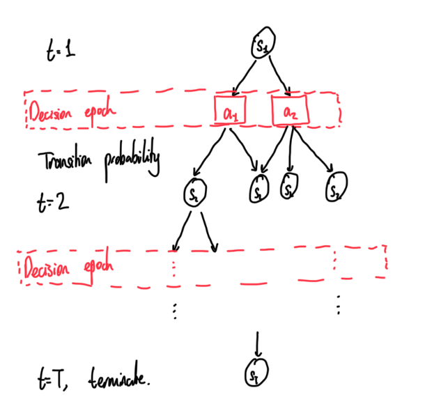
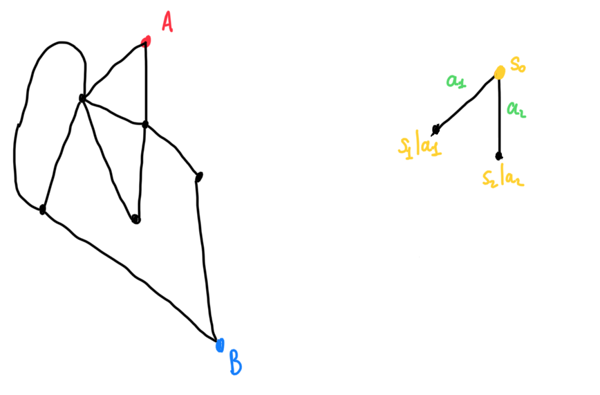
An example of this could be in a shortest path problem. Say we want to get from place A to B within a road network, our decision periods is at each junction where we choose to say either turn left, go straight, or turn right. Each decision may have an influence on future decisions, and so this can be modelled as an MDP.
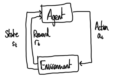
An approach to solving an exact solution to an MDP is by solving the Bellman’s equation, but this is often times very computationally difficult for higher dimensions, as well as requiring knowledge of the model. This is why we want to opt for approximate alternatives which can deal with high dimensions and is model-free. The first approach to this is often a reinforcement learning framework, which models an agent interacting with its environment.
Q-Learning is a common approach to solving MDPs which utilises a form similar to Bellman’s equation, by defining Q(s,a) similar to a value as a function of a state and action pair. This formula is defined by the expected value of the reward after taking the action in the current state, plus the expected value of the rewards in future decision periods,
Q(s,a) = \mathbb{E}\left[\sum_{t=0}^{T} \gamma^t R(s,a) \:|\: s_0 = s, a_0 = a\right].Our goal is to find a Q_*(s,a) which maximises the above function, and the actions associated with the maximum Q. This Q function can be simplified to the form,
Q_*(s,a) = \mathbb{E}\left[R(s,a) + \gamma\max_{a'}Q_*(s',a')\right].This equation can be interpreted as for a given state and action pair, its value is the expected value of reward obtained in the current period, plus the discounted value of all future events given that the optimal action taken. Note that s' and a' denotes the state and action corresponding to the following period.
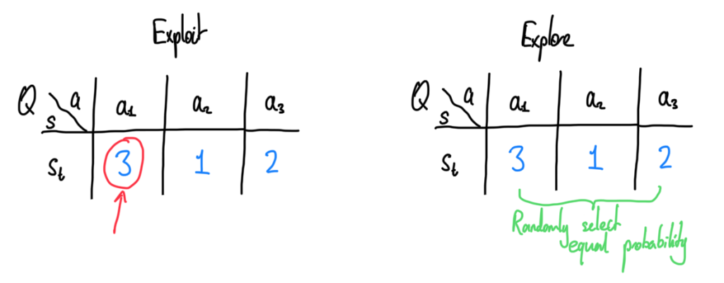
To learn the Q function values, we typically run simulations and adjust our estimates of Q accordingly. In Q-Learning, as opposed to the idea within exact dynamic programming solutions, we focus our exploration on states which are more commonly plausible, but how do we start learning? How do we select our actions taken so we can explore different actions whilst maintaining maximum profits? This problem is commonly referred to as exploration-exploitation trade-off. I will explain the \epsilon-greedy heuristic approach to this problem, but there are a multitude of different methods explored in literature which could be explored in a later blog.
What we do in an \epsilon-greedy framework is to pick based on the Q(s,a) value for a fixed s. The idea is simple, we exploit (pick the best option) with probability \epsilon, and explore with probability 1-\epsilon.
The chosen value for \epsilon \in (0,1] is subjective. One can choose the \epsilon as a constant function, or what is highly recommended often times is to use a form of a decay function, so that we are choosing to explore less and less as we go along. Note however theory says that for convergence of Q-learning to the optimal policy, each state-action pair should be expected to be visited infinitely often.
The most basic form of Q-learning is known as tabular Q-learning. Similar to the above illustration, we would store each Q value within a table corresponding to its current state and its associated action. The initialisation of this is typically using a table of zeroes. Using temporal differencing, we can update the Q function through each iteration based on the observed reward of our current action plus the current optimal action for the future value, compared to the current Q value. Define the Q update as
Q(s,a) \leftarrow Q(s,a) + \alpha\left[R(s,a) + \max_{a'} Q(s',a') - Q(s,a)\right]Here, \alpha is the learning rate parameter, and is a tuneable parameter. We should be careful to set this too high, but it is sufficient in this case to set it as a constant parameter, but one may also choose to set this to a decay function as we may want to learn less over time. For convergence criterion, we only require that \sum_{i=0}^\infty \alpha_i \rightarrow \infty.
And that is it, a simple introduction to tabular Q-learning. The only issue is there are many practical challenges that comes with using Q-learning. First of all, what if there are many state action pairs? Often time we may be required to set the state component into multiple dimensions or we may have a continuous set of actions, therefore memory will play a big part. We will talk more about potential extensions in a second part of Learning About Q-Learning.
Recommended Further Reading Material:
Bertsekas, D. P. (2007). Dynamic Programming and Optimal Control, Vol. I & II. Athena Scientific, Belmont, MA, 3rd edition.
Murphy, K. (2024). Reinforcement learning: An overview. arXiv preprint arXiv:2412.05265.
Sutton, R. S. and Barto, A. G. (2018). Reinforcement Learning: An Introduction. MIT Press, 2nd edition.