The start of the second term of the Master’s year at STOR-i is characterised by a wide range of Research Topics, often shortened to RTs. This begins with eleven days each of which is dedicated to a certain research topic, with around three lectures a day from different researchers in the field. The topics have an even split between Statistics, Operational Research, and the interface between the two areas. Following this, we then have to write two reports, one on a statistical topic, and one on an operational research topic. One of these is a short seven-page report, and the other is a slightly more substantial twenty-page report. For the shorter of these two reports, I opted to look into the area of Computational Statistics, specifically the area of Gaussian Processes.
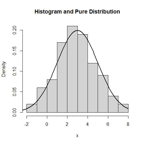
Before we talk about this, we must first introduce the concept of regression. The pure theoretical distributions found in probability are usually described by “parameters”. A simple example is a bell-curve, such as a Normal or t distribution, which will have parameters describing the value about which the distribution is centred, usually the “mean”, and the “scale”, or spread, of the distribution about that data. Some distributions may have a “shape” parameter, which would alter the distribution in a more abstract way. The task of inference is to find the parameters of such a pure distribution such that it matches a real set of data as closely as possible. Note that the choice of distribution itself is a human-made modelling assumption, inference alone cannot choose the right distribution, only the parameters. An example of a “fitted” Normal distribution over some data is given on the left.
The simpler approach to inference is the “Frequentist” approach, whose theory is based on results as the amount of data tends to infinity. Of course, we never have an infinite quantity of data, so inference only ever serves as an approximation to the underlying distribution that produces some set of data. The Frequentist approach assumes that there is one true value for each parameter, and wishes to find said parameter. The alternative approach to inference is the Bayesian approach. As opposed to the Frequentist assumption of one true parameter, Bayesian inference assumes a certain “prior” distribution over each parameter, and updates this distribution into a “posterior” when data is incorporated into the model. This allows for more flexible modelling of uncertainty about parameters with finite data, and also more easily allows this uncertainty to be incorporated into any results.
Counter-intuitively to how we have described inference here, there is also the field of “non-parametric” inference. This name is actually somewhat misleading, as such models can be viewed as treating each piece of observed data as a parameter in its own right. The difference between Frequentist and Bayesian still stands in this case: Frequentist modelling wishes to find the one true underlying answer, whereas the Bayesian approach may obtain infinitely many answers with different probabilities. This difference will be important.
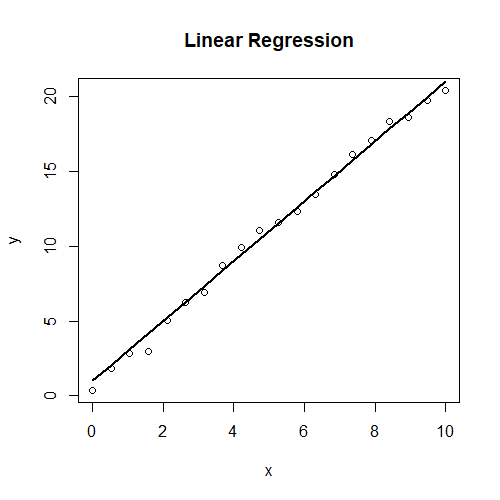
Finally, before finally getting into Gaussian Processes, it’s worth mentioning it’s easier twin: Linear Regression. Linear Regression is best understood as finding a mathematically optimal “line of best fit” for a given set of data (or hyperplane of best fit in higher dimensions). This can be done by putting a parameter on each of the inputs, and adding a random noise term to incorporate randomness. The parameters can then be fitted using either form of inference. An example of this is given on the left, where we assume a model Y = ax + b + e, where a and b are parameters and e is a random noise term. a and b are then fitted to be around 2 and 1 respectively, matching the data. However, a more difficult task is non-linear regression, where the observed data given the inputs could be generated by any underlying function, not just a linear one. This is where Gaussian Processes come into use.
Gaussian Process Regression is a Bayesian non-parametric approach to non-linear regression. That is to say, it considers each point of observed data to be its own parameter, and gives back a class of possible functions (not just a single answer) which pass through or near the observed data. To build up to the idea of a Gaussian Process, we can first describe a Multivariate Normal distribution. Consider two random variables X and Y both of which are Normal, and which may or may not be related in some way. The vector (X,Y) is then a multivariate random variable whose parameters include the mean and the “covariance matrix”. The mean is simply the vector of means of X and Y, and the covariance matrix is a structure which contains information on the variance of X and Y in isolation, and information on how they interact with each other. This notion can be extended to any finite dimension. A Gaussian Process, in general, is any collection of random variables (in our case, uncountably infinitely many) where any finite subset of these variables is a multivariate normal. That is to say, if \(\) f [\latex] is a Gaussian Process, f(x) is a Normal distribution for any real-valued x, and any finite vector f(x)s evaluated at different xs gives a Multivariate Normal distribution. A sample from a Gaussian Process is then a function. A Gaussian Process can be uniquely characterised by a “mean function” to describe the central trend, and a two-input “kernel” function which describes the covariance (dependence structure) between any two f(x) and f(y). The technicalities of choosing a class of kernels for regression will be avoided here, but a good way of understanding the choice of a kernel function is how “smooth” you expect the underlying functions to be. To complicate matters further, kernels have “hyperparameters” which also have the be optimised.
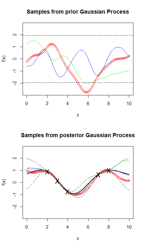
On the left we give some examples of samples from Gaussian Processes. The first image shows approximate sample functions from the prior Gaussian Process, using what is known as the Squared Exponential kernel. In short, this kernel enforces a strict smoothness condition which, for those familiar with calculus, only allows for infinitely differentiable functions. In short, this means no sharp points or quick turns are permitted. We say “approximate” sample functions because, in reality, we only evaluate a sample function at finitely many points at a time, as shown explicitly by the red points. The dashed black lines give “confidence intervals”, giving the bounds in which we usually expect a function to remain within. However, when a function does leave those bounds, we expect it to leave those bounds for a given interval due to the smoothness of the function guaranteed by the smooth kernel. That is, sudden “spikes” out of the bounds are not permitted.
The second image demonstrates how the process behaves once it has observed some data. Clearly, this data is non-linear (and was in fact generated from a sine wave). We see that the sample functions now behave far more similarly to each other within the range of the data, and the confidence intervals have tightened significantly around areas where there is data. Intuitively, this appears to be a very satisfactory example of a successful non-linear regression. However, it is worth noting the wide confidence intervals to the left of the lowest point and to the right of the highest point. In absence of data, the posterior degrades back into the prior, demonstrating that Gaussian Process Regression is good for interpolating within the data, but not outside it.
We have demonstrated that Gaussian Process Regression is a powerful tool for interpolating non-linear data. However, it has even broader applications. For example, Gaussian Processes can be extended to nodes on a network structure, in such a way that the kernel can integrate the structure of the network into the process, as demonstrated in Matérn Gaussian Processes on Graphs (Borovitskiy et al., 2021). It can also be used for the task of “classification”. In short, linear classification uses a linear model to measure how much a given input falls into a certain “class”, and this linear model is then “flattened” between 0 and 1 using a sigmoid function (S-shaped function), and the result can be interpreted as the probability that the input belongs to a given class. A simple example would be a model that takes an image as an input (each pixel would be represented by one value), and returns the probability that the image is a cat (note that a simple linear model would not be capable of this, it’s just an example of a classification problem generally speaking). A generalisation of this approach would use a non-linear function which is then flattened between 0 and 1, and this general function could be modelled using a Gaussian process.
A final example of how Gaussian processes can be used is in optimisation. The field of Bayesian Optimisation considers that problem of finding the input that maximises a function that is “expensive” to compute. For example, this function may be some complex computer simulation that takes some input, and returns some performance metric that we wish to maximise or minimise. Starting with a few function evaluations, a Gaussian process can be used to approximate how the function behaves in between the evaluated points, and can then also be used to work out where it is best to evaluate the function next. There are many approaches to this, but all use the common theme of “exploitation and exploration”, which seeks to find a balance between exploring areas of the function with little information and high variance (exploration) and fine tuning areas of the function which are already showing good results (exploitation).
In short, Gaussian Processes are a powerful tool for non-linear regression and interpolating data in a way that is very flexible and which can quantify its own uncertainty, making it a very useful tool for approximating trends, classification, and optimisation. For those wishing to look further into Gaussian processes, I recommend “Gaussian Processes for Machine Learning” (Rasmussen and Williams, 2006), which can be found online for free.
Very nice article, totally what I was looking for.