Home page for accesible maths 6 Linear transformations 6.1 Definition and first examples 6.3 Invertible linear transformations

Style control - access keys in brackets

Font (2 3) - + Letter spacing (4 5) - + Word spacing (6 7) - + Line spacing (8 9) - +

6.2. Linear transformations versus matrices

The purpose of this section is to emphasize the following correspondence:

Linear transformations

T

Composition of functions,

T\circ S

T\begin{pmatrix}x\\ y\end{pmatrix}

\displaystyle\longleftrightarrow\framebox{ \begin{tabular}[]{c}Matrices\\ $A$\\ Matrix multiplication, $AB$\\ $\begin{pmatrix}a_{11}&a_{12}\\ a_{21}&a_{22}\end{pmatrix}\begin{pmatrix}x\\ y\end{pmatrix}$\end{tabular}}

For every linear transformation we will assign exactly one matrix to it (Definition 6.2.5), and for every matrix there is exactly one linear transformation which it defines (Example 6.1). This type of correspondence is called a bijection or a bijective correspondence, and above this is indicated by the two-way array $\leftrightarrow$ .

An advantage of writing transformations using matrices is that it makes some computations easier; for example, composition of maps is given by matrix multiplication. If $T_{A},T_{B}$ are transformations with matrices $A, B$ respectively, then the composition $T_{A}\circ T_{B}$ is equal to $T_{AB}$ . This is, in fact, the reason why matrix multiplication is defined the way it is.

Recall that composition of maps reads right to left, i.e. $T_{A}\circ T_{B}$ means ‘first do $T_{B}$ , then $T_{A}$ ’. This matters because in general $T_{B}\circ T_{A}\neq T_{A}\circ T_{B}$ . For convenience, we often write $T_{A}T_{B}$ instead of $T_{A}\circ T_{B}$ .

Example 6.2.1.

Consider the following matrices:

$A:=\begin{pmatrix}1&2\\ 0&1\end{pmatrix},\quad B:=\begin{pmatrix}0&3\\ -1&0\end{pmatrix}.$

Then their associated linear transformations can be written as

$T_{A}(x,y)=(x+2y,y),\quad T_{B}(x,y)=(3y,-x).$

Let’s calculate the composition:

$(T_{A}\circ T_{B})(x,y)=T_{A}(3y,-x)=(3y-2x,-x).$

This is the linear transformation associated to the matrix $AB=\begin{pmatrix}-2&3\\ -1&0\end{pmatrix}$ , as expected.

Throughout this section, we consider the Euclidean plane ${\mathbb{R}}^{2}$ , and transformations ${\mathbb{R}}^{2}\to{\mathbb{R}}^{2}$ . But you should know that linear transformations ${\mathbb{R}}^{n}\to{\mathbb{R}}^{m}$ correspond to $m\times n$ matrices in exactly the same way. We will look at the $\operatorname{M}_{{2}}({{\mathbb{R}}})$ case because it is easiest to visualise.

The standard basis vectors of ${\mathbb{R}}^{2}$ are $\{e_{1},e_{2}\}$ (See Definition 1.4.8). So we have already two equivalent ways of writing the same vector, given by the left and right hand sides of the following equation:

\begin{pmatrix}a\\ b\end{pmatrix}=ae_{1}+be_{2}.

We will use the following notation for points in ${\mathbb{R}}^{2}$ :

(a,b)\in{\mathbb{R}}^{2}.

Notice this notation is different from the $1\times 2$ matrix $\begin{pmatrix}a&b\end{pmatrix}$ because of the comma.

Remark 6.2.2.

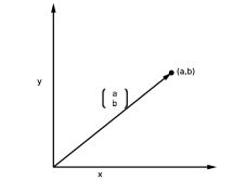
Points and vectors in ${\mathbb{R}}^{n}$ can be identified with each other. Explicitly, a point $P=(x,y)$ corresponds to the vector from $O$ to $P$ , $\vec{OP}=\begin{pmatrix}x\\ y\end{pmatrix}$ , where $O=(0,0)$ (see Figure 4). Thus, the convention is that we write the coordinates of points horizontally with commas between them, and the vectors vertically, as column vectors. In practice, it is usually okay to equate the two in your head. We use the notation to emphasize the different perspectives of “vectors” versus “points”, and it is common to switch between the two.

Figure 4. The vector and point corresponding to the pair $(a,b)\in{\mathbb{R}}^{2}$

Proposition 6.2.3.

Let $T_{1},T_{2}:{\mathbb{R}}^{2}\to{\mathbb{R}}^{2}$ be linear transformations. Then the composition $T_{2}T_{1}$ is also a linear transformation.

Proof.

Let $\lambda\in{\mathbb{R}}$ and pick any vectors $v,w\in{\mathbb{R}}^{2}$ . We have

	$\displaystyle T_{2}T_{1}(v+w)$	$\displaystyle=T_{2}\big{(}T_{1}(v+w)\big{)}=T_{2}\big{(}T_{1}(v)+T_{1}(w)\big{)}$	$\displaystyle\quad\hbox{since $T_{1}$ is linear}$
		$\displaystyle=T_{2}\big{(}T_{1}(v)\big{)}+T_{2}\big{(}T_{1}(w)\big{)}$	$\displaystyle\quad\hbox{since $T_{2}$ is linear}$
		$\displaystyle=T_{2}T_{1}(v)+T_{2}T_{1}(w)$
and
	$\displaystyle T_{2}T_{1}(\lambda v)$	$\displaystyle=T_{2}\big{(}T_{1}(\lambda v)\big{)}=T_{2}\big{(}\lambda T_{1}(v)% \big{)}$	$\displaystyle\quad\hbox{since $T_{1}$ is linear}$
		$\displaystyle=\lambda T_{2}\big{(}T_{1}(v)\big{)}$	$\displaystyle\quad\hbox{since $T_{2}$ is linear}$
		$\displaystyle=\lambda T_{2}T_{1}(v)$

which proves that LT1 and LT2 hold. ∎

Theorem 6.2.4.

Any linear transformation of ${\mathbb{R}}^{2}$ is determined by its effect on the standard basis vectors $e_{1}$ and $e_{2}$ . In other words, a linear transformation $T$ is entirely known if $T(e_{1})$ and $T(e_{2})$ are given.

Proof.

Since any vector can be written in the form $ae_{1}+be_{2}$ , where $a,b\in{\mathbb{R}}$ , by linearity we have $T(ae_{1}+be_{2})=aT(e_{1})+bT(e_{2})$ . ∎

Definition 6.2.5.

Given a linear transformation $T$ of ${\mathbb{R}}^{2}$ , and let $a_{11},a_{12},a_{21},a_{22}\in{\mathbb{R}}$ be defined as

T(e_{1})=a_{11}e_{1}+a_{21}e_{2}\quad\hbox{and}\quad T(e_{2})=a_{12}e_{1}+a_{2% 2}e_{2}.

The matrix $A=\begin{pmatrix}a_{11}&a_{12}\\ a_{21}&a_{22}\end{pmatrix}$ is called the matrix associated to the linear transformation $T$ .

Remark 6.2.6.

•

There is nothing special about the ${\mathbb{R}}^{2}$ case here; this definition could be generalised to higher dimensions.
•

In fact, $A$ is the matrix of $T$ with respect to the standard basis $\{e_{1},e_{2}\}$ of ${\mathbb{R}}^{2}$ . In more general situations, such as in MATH220, one could use a different basis, which would produce a different matrix.
•

We will also say that $T$ is the linear transformation given by the matrix $A$ .

Theorem 6.2.7.

Let $A$ , $B$ be the matrices of the linear transformations $T$ and $S$ of ${\mathbb{R}}^{2}$ . Then

(i)

$T\begin{pmatrix}x\\ y\end{pmatrix}=\begin{pmatrix}a_{11}&a_{12}\\ a_{21}&a_{22}\end{pmatrix}\begin{pmatrix}x\\ y\end{pmatrix}=A\begin{pmatrix}x\\ y\end{pmatrix}$ .
(ii)

$A B$ (matrix multiplication) is the matrix of the linear transformation $T\circ S$ .

Proof.

We have that $\begin{pmatrix}x\\ y\end{pmatrix}=xe_{1}+ye_{2}$ . Thus

$\displaystyle T(xe_{1}+ye_{2})$	$\displaystyle=xT(e_{1})+yT(e_{2})$	$\displaystyle\quad\text{by linearity}$
	$\displaystyle=x(a_{11}e_{1}+a_{21}e_{2})+y(a_{12}e_{1}+a_{22}e_{2})$	$\displaystyle\quad\text{by Definition~{}\ref{def:ltmatrix}}$
	$\displaystyle=(xa_{11}+ya_{12})e_{1}+(xa_{21}+ya_{22})e_{2}$
	$\displaystyle=\begin{pmatrix}a_{11}x+a_{12}y\\ a_{21}x+a_{22}y\end{pmatrix}=\begin{pmatrix}a_{11}&a_{12}\\ a_{21}&a_{22}\end{pmatrix}\begin{pmatrix}x\\ y\end{pmatrix}$	$\displaystyle\quad\text{by Definition~{}\ref{def:matrixvector}.}$

This proves part (i).

For part (ii), let $C$ be the matrix of $T\circ S$ , which is a linear transformation by Proposition 6.2.3. So

T(S(e_{1}))=(T\circ S)(e_{1})=c_{11}e_{1}+c_{21}e_{2}.

On the other hand, we have that

$\displaystyle T(S(e_{1}))$	$\displaystyle=T(b_{11}e_{1}+b_{21}e_{2})$	$\displaystyle\quad\hbox{since $B$ is the matrix for $S$}$
	$\displaystyle=b_{11}T(e_{1})+b_{21}T(e_{2})$	$\displaystyle\quad\hbox{by linearity of $T$}$
	$\displaystyle=b_{11}(a_{11}e_{1}+a_{21}e_{2})+b_{21}(a_{12}e_{1}+a_{22}e_{2})$
	$\displaystyle=(a_{11}b_{11}+a_{12}b_{21})e_{1}+(a_{21}b_{11}+a_{22}b_{21})e_{2}.$

Equating coefficients of $e_{1}$ , we find that $c_{11}=a_{11}b_{11}+a_{12}b_{21}$ , while equating coefficients of $e_{2}$ , we get $c_{21}=a_{21}b_{11}+a_{22}b_{21}$ . A similar calculation for $T(S(e_{2}))$ gives expressions for $c_{12}$ and $c_{22}$ in terms of $a_{11},\ldots,a_{22}$ and $b_{11},\ldots,b_{22}$ , and in all four cases we see that $c_{ij}$ is equal to the $(i,j)$ coefficient of the matrix product $A B$ defined in Definition 1.4.1; that is, $C=AB$ . ∎

Proposition 6.2.8 (Rotation transformations).

In coordinates, anticlockwise rotation through the angle $\theta$ is given by

R_{\theta}(x,y)=(~{}x\cos\theta-y\sin\theta\quad\hbox{,}\quad x\sin\theta+y% \cos\theta~{})\quad\hbox{for all $(x,y)\in{\mathbb{R}}^{2}.$}\quad

So a rotation around the origin is represented by the matrix

R_{\theta}=\begin{pmatrix}\cos\theta&-\sin\theta\\ \sin\theta&\cos\theta\end{pmatrix}.

In particular, it is a linear transformation.

Proof.

Assume the vector $v=\begin{pmatrix}x\\ y\end{pmatrix}$ makes an angle $\alpha$ above the positive $x$ -axis. The length of $v$ is $r=\sqrt{x^{2}+y^{2}}$ (see Definition 1.3.5), so we can use polar coordinates to write $P=(x,y)=(r\cos\alpha,r\sin\alpha)$ . When $P^{\prime}$ is written in polar coordinates, it makes an angle $\alpha+\theta$ with the $x$ -axis, so we have $P^{\prime}=(x^{\prime},y^{\prime})=(r\cos(\alpha+\theta),r\sin(\alpha+\theta))$ . Now we can use trigonometric identities as follows:

	$\displaystyle x^{\prime}$	$\displaystyle=r\cos(\alpha+\theta)=r(\cos\theta\cos\alpha-\sin\theta\sin\alpha)$
		$\displaystyle=(r\cos\alpha)\cos\theta-(r\sin\alpha)\sin\theta$
		$\displaystyle=x\cos\theta-y\sin\theta$
and
	$\displaystyle y^{\prime}$	$\displaystyle=r\sin(\alpha+\theta)=r(\sin\theta\cos\alpha+\cos\theta\sin\alpha)$
		$\displaystyle=(r\cos\alpha)\sin\theta+(r\sin\alpha)\cos\theta$
		$\displaystyle=x\sin\theta+y\cos\theta.$

This proves the results. ∎

Proposition 6.2.9 (Reflection transformations).

In coordinates, the reflection about the line $l_{\theta}$ , whose angle above the $x$ -axis is $\theta$ , is given by

H_{\theta}(x,y)=(~{}x\cos 2\theta+y\sin 2\theta~{},~{}x\sin 2\theta-y\cos 2% \theta~{})\quad\hbox{for all $(x,y)\in{\mathbb{R}}^{2}.$}\quad

So it may be represented by the matrix

H_{\theta}=\begin{pmatrix}\cos{2\theta}&\sin{2\theta}\\ \sin{2\theta}&-\cos{2\theta}\end{pmatrix}.

In particular, it is a linear transformation.

Proof.

Let $P^{\prime}=(x^{\prime},y^{\prime})$ be the image of $P=(x,y)\in{\mathbb{R}}^{2}$ , as in Figure 3. If the vector corresponding to $P$ makes an angle $\alpha$ above the $x$ -axis, then the angle between $l$ and $v$ is $\theta-\alpha$ . Therefore, $P^{\prime}$ is obtained from $P$ by a rotation through $2(\theta-\alpha)$ . So the angle $P^{\prime}$ makes with the $x$ -axis is $2(\theta-\alpha)+\alpha=2\theta-\alpha$ . Therefore, using trigonometric identities and polar coordinates (see the rotational case above),

	$\displaystyle x^{\prime}$	$\displaystyle=r\cos(2\theta-\alpha)=r(\cos 2\theta\cos\alpha+\sin 2\theta\sin\alpha)$
		$\displaystyle=x\cos 2\theta+y\sin 2\theta$
and
	$\displaystyle y^{\prime}$	$\displaystyle=r\sin(2\theta-\alpha)=r(\sin 2\theta\cos\alpha-\cos 2\theta\sin\alpha)$
		$\displaystyle=x\sin 2\theta-y\cos 2\theta.$

∎

Now we have seen the examples of the rotation around the origin, and of a reflection about a line. We found that for any angle $\theta\in[0,2\pi)$ , they are represented by the matrices

R_{\theta}=\begin{pmatrix}\cos\theta&-\sin\theta\\ \sin\theta&\cos\theta\end{pmatrix}\quad\hbox{and}\quad H_{\theta}=\begin{% pmatrix}\cos 2\theta&\sin 2\theta\\ \sin 2\theta&-\cos 2\theta\end{pmatrix}.

We showed this by using trigonometric identities. But there is a faster geometric way: consider the Figures 2 and 3, and see where $e_{1}$ and $e_{2}$ are mapped:

	$\displaystyle R_{\theta}(e_{1})=\begin{pmatrix}\cos\theta\\ \sin\theta\end{pmatrix},$	$\displaystyle R_{\theta}(e_{2})=\begin{pmatrix}-\sin\theta\\ \cos\theta\end{pmatrix}$
	$\displaystyle H_{\theta}(e_{1})=\begin{pmatrix}\cos 2\theta\\ \sin 2\theta\end{pmatrix},$	$\displaystyle H_{\theta}(e_{2})=\begin{pmatrix}\sin 2\theta\\ -\cos 2\theta\end{pmatrix}.$

So the matrices we found in Propositions 6.2.8 and 6.2.9 are correct.

Example 6.2.10.

Prove that we have the equality $R_{\pi/3}H_{0}=H_{\pi/6}$ .
Solution: The LHS is the composition of the reflection about the $x$ -axis followed by the anticlockwise rotation through $\frac{\pi}{3}$ , while the RHS is the reflection about the line which makes an angle $\frac{\pi}{6}$ with the $x$ -axis. To prove the claim, let us calculate with their associated matrices:

$R_{\pi/3}H_{0}=\begin{pmatrix}\frac{1}{2}&-\frac{\sqrt{3}}{2}\\ \frac{\sqrt{3}}{2}&\frac{1}{2}\end{pmatrix}\begin{pmatrix}1&0\\ 0&-1\end{pmatrix}=\begin{pmatrix}\frac{1}{2}&\frac{\sqrt{3}}{2}\\ \frac{\sqrt{3}}{2}&-\frac{1}{2}\end{pmatrix}=\begin{pmatrix}\cos\frac{\pi}{3}&% \sin\frac{\pi}{3}\\ \sin\frac{\pi}{3}&-\cos\frac{\pi}{3}\end{pmatrix}=H_{\pi/6}.$

Their associated matrices are equal, and therefore these linear transformations are equal.