III Quantum information representation and manipulation

Quantum computers encode information into the quantum state of a composite system, consisting of a number of two-state systems known as qubits (quantum bits). Taken individually, each qubit can be described by a quantum state $|\psi ⟩=\alpha |0⟩+\beta |1⟩$. The basis states $|0⟩$ and $|1⟩$ form the computational basis, and represent classical bits with values 0 and 1. What is special about qubits is that their general state $|\psi ⟩$ can also be a superposition of 0 and 1, which cannot be realized by a classical bit. In this case, ${|\alpha |}^2$ and ${|\beta |}^2$ give the probabilities to find 0 or 1 in a measurement of the qubit in the computational basis [associated with the operator $(I-Z)/2$], which on the Bloch sphere depend on the polar angle $\theta$. Measurements of other observables (like $X$ or $Y$) give access to other combinations of $\alpha$ and $\beta$, which also depend on the phase $\varphi =\arg ({\alpha }^{*}\beta )$ of the qubit. However, since measurements change the state of the qubit, it is not possible to directly encode information into the complex numbers $\alpha$ and $\beta$; this distinguishes quantum computers from analog computers.

An $N$-bit quantum register contains $N$ qubits. The state of the register is then formed using the $𝒩=2^N$ computational basis states $|x_{N-1}\mathrm{\dots }{x}_1{x}_0⟩$, where $x_{N-1}\mathrm{\dots }{x}_1{x}_0$ is the binary code of numbers $x={\sum }_{n=0}^{N-1}{x}_n{2}^n$ ranging from $0$ to $2^N-1$. Here, we will not drop leading zeros (thus, for $N=4$ we write 0010 for the decimal number 2) because they describe the state of some of the qubits. Sometimes, we denote these states by the corresponding numbers $x$; e.g., for a 4-bit register, $|3⟩\equiv |0011⟩$ and $|0⟩\equiv |0000⟩$.

Just as the individual qubits, the register may be brought into a superposition of the computational basis states. For instance, one can form the state

$$|\mathrm{\Psi }⟩\equiv 2^{-N/2}\sum _{x_n=0,1}|x_{N-1}\mathrm{\dots }{x}_1{x}_0⟩=2^{-N/2}\sum _{x=0}^{2^N-1}|x⟩,$$

which contains all binary numbers between 0 and $2^N-1$ at the same time. All these numbers therefore can be manipulated at once by a single physical operation on the register. This feature is sometimes described as quantum parallelism, and will be frequently exploited in Section V.

The state $|\mathrm{\Psi }⟩$ given above is still separable, and therefore can be obtained by operating on the individual qubits. The real power of the register is unleashed when one considers that the qubits in the register can also be entangled, which can be achieved by manipulating pairs of qubits. We next explore how entanglement is linked to information and then have a look at a number of basic quantum operations on the register which enable to exploit these special features of qubits.

Quantum mechanically, the entropy of a system with density matrix $\widehat{\rho }$ is given by the von Neumann entropy

$$S(\widehat{\rho })=-\mathrm{tr}\widehat{\rho }{\log }_2\widehat{\rho }.$$

This is identical to the Shannon entropy, with the probabilities $p_n$ replaced by the eigenvalues of $\widehat{\rho }$. It follows that a system in a pure state has von-Neumann entropy $S=0$.

Classically, the entropy of a subsystem $A$ is always less than the entropy of a composite system with parts $A$ and $B$: . Quantum mechanically, the entropy $S({\widehat{\rho }}_A)$ of a subsystem follows by inserting the reduced density matrix, and can be larger than the entropy of a composed system. This is in particular the case when an entangled systems is in a pure state. The entropy of the composite system vanishes, but it is finite for each of its parts because the reduced density matrices are mixed (see section I.7). For composite systems that are already in a mixed state, this leads to the more sophisticated measures of entanglement also mentioned in that section.

In terms of data compression, the von Neumann entropy plays a similar role as the Shannon entropy: it describes how many qubits are necessary to transmit a certain amount of (quantum) information (this can be quantified via Schumacher’s noiseless channel coding theorem).

How much information can be transmitted via a single qubit? Assume that the incoming data stream is composed of states described by a density matrix ${\widehat{\rho }}_i$, which can be assumed to be mixed because of limitations in the preparation or transmission of the qubit states. It then can be shown that the maximally accessible amount of information $I$ per qubit cannot exceed a certain limit, , where $\widehat{\rho }={\sum }_i{P}_i{\widehat{\rho }}_i$, and $P_i$ is the fraction of qubits with density matrix ${\widehat{\rho }}_i$. This inequality is known as the Holevo bound, and the quantity $\chi$ is the Holevo information. Note that when all ${\widehat{\rho }}_i$ are pure, $S({\widehat{\rho }}_i)=0$, and therefore $\chi =S(\widehat{\rho })$.

The Holevo bound implies that a single qubit cannot transmit more than one bit of classical information. However, as embodied by the superdense coding scheme discussed next, if sender and receiver possess as an additional resource a number of shared entangled qubits, it is possible to transmit two bits of classical information via a single (entangled) qubit. Indeed, the applications below show that entanglement is a useful, non-classical resource for communication. Entanglement can also be used for error correction schemes, as will be discussed in section VI.1.

In order to quantify entanglement of a (many-body) state $|\psi ⟩$, it is useful to determine how many maximally entangled Bell pairs one could generate (by local operations within each subsystem, and classical communication) if one had many copies of the state $|\psi ⟩$. This results in the entanglement of formation, which is an additive measure of entanglement, and therefore constitutes the appropriate counterpart to the information measure provided by the Shannon entropy. As discussed in Sec. I.7, for pure states the entanglement of formation simply reduces to the von Neumann entropy of the subsystems. This applies even for the case that each subsystem has more than two possible quantum states. For mixed states, however, explicit expressions are only known for some special cases, such as for two qubit-systems (see again Sec. I.7).

Since solutions of the Schrödinger equation can be written as a time-dependent unitary transformation of the initial state, all quantum gates are represented by unitary operators, $|{\psi }_{\mathrm{f}}⟩=\widehat{U}|{\psi }_{\mathrm{i}}⟩$, where $|{\psi }_{\mathrm{i}}⟩$ is the initial state of the register, and $|{\psi }_{\mathrm{f}}⟩$ is the final state of the register. Computational algorithms furthermore complement these gates by mechanisms to prepare the register in an initial state, as well as mechanisms to read out the final state (which can be achieved by measurements). In the remainder of this section we concentrate on the unitary quantum gates.

First, a general observation: Because unitary operators can be inverted, all quantum gates are reversible: the input state can be inferred from $|{\psi }_{\mathrm{i}}⟩={\widehat{U}}^{†}|{\psi }_{\mathrm{f}}⟩$. This also entails an important constraint onto quantum operations: The no-cloning theorem, according to which it is impossible to transfer the state of a control qubit to a target qubit without erasing the state of the control qubit.

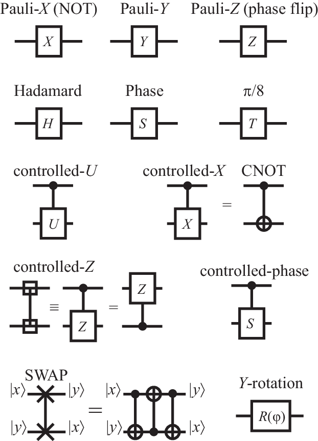
Even though the quantum gates are reversible, a universal set of gates can be formed using only unary and binary gates; no three-bit gates are required. On the other hand, we need to consider a larger variety of such gates — besides achieving the classical logical tasks, we need gates that put qubits into non-classical superpositions of 0 and 1, and gates that establish entanglement between the qubits. Fortunately, this can be achieved by using a finite number of unary gates, plus a single binary gate. Circuit representations of these gates are shown in Fig. 3.

All unary (single-qubit) gates can be represented as $2\times 2$-dimensional unitary matrices, which act on the two component vector $\psi =\left(\begin{array}{c}\hfill \alpha \hfill \\ \hfill \beta \hfill \end{array}\right)$ representing the state $|\psi ⟩=\alpha |0⟩+\beta |1⟩$. Just as hermitian matrices, these can be generated by combining the Pauli matrices $X$, $Y$, and $Z$, as well as the identity matrix $I$. The latter leaves the state of the qubit unchanged, and therefore constitutes the quantum analogue to the identity gate $\mathrm{Id}$. Furthermore, considering that $X|0⟩=|1⟩$ and $X|1⟩=|0⟩$, $X$ represents the analogue to the classical NOT gate. For a general state $|\psi ⟩=\alpha |0⟩+\beta |1⟩$ of the qubit, application of this gate yields $X|\psi ⟩=\beta |0⟩+\alpha |1⟩$. Because they are irreversible, the two remaining classical unary gates ALWAYS TRUE/FALSE do not have unary quantum analogues.

Clearly, $I$ and $X$ do not exhaust all possible transformations of a qubit. On the Bloch sphere, $X$ represents a rotation by 180${}^{\circ }$ about the $x$ axis, while $I$ leaves the state untouched. However, we can also operate, e.g., with $Z$, which flips the phase of the qubit (this advances the azimuthal angle $\varphi$ by $\pi$). The most general single-qubit transformations correspond to rotations of the Bloch sphere about an arbitrary axis $\widehat{𝐧}=(n_x,n_y,n_z)$, by an arbitrary angle $\phi$. Such general rotations can be written as

	$R_{\widehat{𝐧}}(\phi )$	$=$	$\exp [-i\phi (n_{x}X+n_{y}Y+n_{z}Z)/2]$
		$=$	$\cos (\phi /2)I-i\sin (\phi /2)(n_{x}X+n_{y}Y+n_{z}Z).$

Fortunately, not all rotations are independent: E.g., following from the identity $Y=iXZ$, $Y$ (a 180${}^{\circ }$ rotation about the $y$ axis) can be obtained by combining $X$ and $Z$ (rotations about the $x$ and $z$ axis, respectively).

An example of a set of elementary rotations which can be combined to generate all possible rotations is given by the following three gates: the $\pi /8$-gate

the phase gate

and the Hadamard gate

Here, $T$ and $S$ generate ${45}^{\circ }$ and ${90}^{\circ }$ rotations about the $z$ axis, respectively, while $H$ generates a ${180}^{\circ }$ rotation about the $(1,0,1)$ direction. Starting, say, from the initial state $|0⟩$, these operations can be used to bring the qubit into any general superposition state $\alpha |0⟩+\beta |1⟩$.

Below, we will also often use $\phi$-rotation gates about the $Y$ axis, which have the form

General two-qubit gates are represented by $4\times 4$-dimensional unitary matrices, which act on the four component vector

$$\psi =\left(\begin{array}{c}\hfill \alpha \hfill \\ \hfill \beta \hfill \\ \hfill \gamma \hfill \\ \hfill \delta \hfill \end{array}\right)$$

representing a state $|\psi ⟩=\alpha |00⟩+\beta |01⟩+\gamma |10⟩+\delta |11⟩$.

The most important gate is the quantum version of the controlled-not gate CNOT, which negates the target qubit if the control qubit is in $|1⟩$, and leaves the target unchanged if the control qubit is in $|0⟩$; the control qubit always remains in its initial state. If qubit 1 is the control bit, this is represented by the matrix

for reversed roles we have

Starting, say, from the separable state $|\psi ⟩=\sqrt{1/2}(|0⟩+|1⟩)|0⟩=\sqrt{1/2}(|00⟩+|10⟩)$, we find $C_{12}|\psi ⟩=\sqrt{1/2}(|00⟩+|11⟩)$, i.e., one of the Bell states. The CNOT gate can therefore be used to entangle two qubits.

In block notation, the matrix $C_{12}$ can also be written as . Replacing $X$ by an arbitrary unary gate $U$ delivers controlled versions of each unary gate, denoted as controlled-$U$ gates. An example is the controlled phase flip, which is obtained for $U=Z$. Another notable two-qubit gate is the quantum version of the SWAP gate, which is represented by the matrix

In order to manipulate the information in the register, we need to apply unary and binary gates to the individual qubits. Unary gates $U$ operating on the $n$th qubit in the register will be denoted by $U_n$. Analogously, binary gates acting on qubits $n$ and $m$ will be denoted by $U_{nm}$. Here, order of the indices matters — in general, $U_{nm}\ne U_{mn}$. In particular, for controlled gates, we will use the first index to refer to the control qubit, while the second index refers to the target qubit.

We can now combine unary and binary gates to achieve arbitrary operations on the register. For instance, the realization of the SWAP gate in terms of three CNOT gates, already known from the classical case, takes the form $S_{12}=C_{12}{C}_{21}{C}_{12}$.

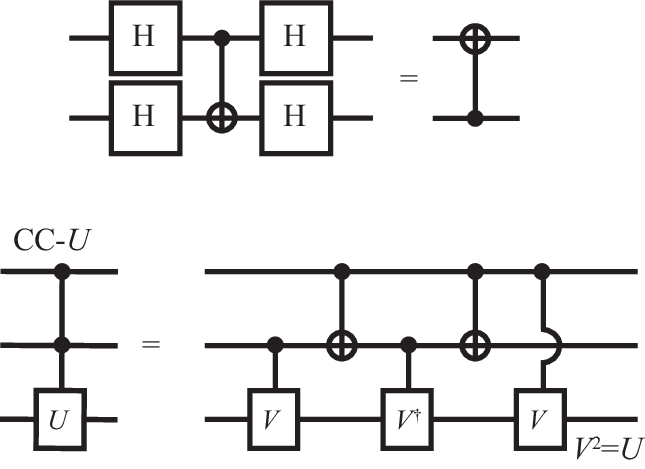
The combination of quantum gates allows to achieve tasks that would require more complicated gates if done classically. Some examples are listed in Fig. 4. Consider the operation $U=H_1{H}_2{C}_{12}{H}_1{H}_2$, which first applies Hadamard gates to the two qubits, then acts with a CNOT gate, and finally again applies Hadamard gates. Using matrix multiplications, we find that for all initial states, this is equivalent to $U=C_{21}$. Therefore, amazingly, decorating the gate with single-qubit operations allows to exchange the roles of the control and target qubits. Classically, this exchange would require additional binary gates. Similarly, we can obtain classical three-bit gates by combination of unary and binary gates. For instance, as shown in the figure, a general controlled-controlled-$U$ gate can be obtained by controlled-$V$ gates, where $V^2=U$.

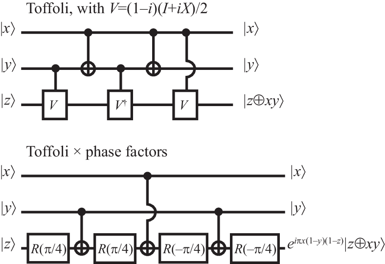
The Toffoli gate (controlled-controlled-not, CCNOT), which classically has to be introduced separately to achieve unversal reversible computations, follows for $V=(1-i)(I+iX)/2$, such that $V^2=X$. Just as in the classical case, the Fredkin gate is obtained by two additional CNOT operations, $F_{123}=C_{32}{T}_{123}{C}_{32}$. Up to a phase factor, the Toffoli gate can also be achieved by using $Y$-rotations,

$$e^{i\vartheta }{T}_{123}=R_3(-\pi /4)C_{13}{R}_3(-\pi /4)C_{23}{R}_3(\pi /4)C_{13}{R}_3(\pi /4)$$

(see Fig. 5). Here, the phase factor $\vartheta$ changes the sign of the basis state $|100⟩$, but leaves all other basis states unchanged.

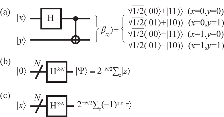
Figure 6 shows combinations of gates which serve as frequent components of the quantum algorithms discussed in the following section. (a) The gate $C_{12}{H}_1$ entangles qubits $1$ and $2$ that are initially prepared in computational basis states:

	$C_{12}{H}_1|00⟩=\sqrt{1/2}(|00⟩+|11⟩)\equiv |{\beta }_{00}⟩,$
	$C_{12}{H}_1|01⟩=\sqrt{1/2}(|01⟩+|10⟩)\equiv |{\beta }_{01}⟩,$
	$C_{12}{H}_1|10⟩=\sqrt{1/2}(|00⟩-|11⟩)\equiv |{\beta }_{10}⟩,$
	$C_{12}{H}_1|11⟩=\sqrt{1/2}(|01⟩-|10⟩)\equiv |{\beta }_{11}⟩.$

(b) Application of $U={\prod }_n{H}_n$ (i.e., acting with the Hadamard gate on each qubit) transforms an $N$-qubit register with initial state $|0⟩=|000\mathrm{\dots }000⟩$ into

$$U|\psi ⟩=2^{-N/2}\sum _{x_n=0,1}|x_{N-1}\mathrm{\dots }{x}_2{x}_1{x}_0⟩\equiv |\mathrm{\Psi }⟩,$$

the superposition of all states of the computational basis, which represents all binary numbers in the range of the register. (c) When the initial state is another computation basis state $|x⟩$, the action of a Hadamard gate on an individual qubit can be written as

$$H|x_n⟩=\frac{|0⟩+{(-1)}^{x_n}|1⟩}{\sqrt{2}}=\frac{1}{\sqrt{2}}\sum _{z_n=0,1}{(-1)}^{x_n{z}_n}|z_n⟩.$$

When we act with Hadamard gates on all the qubits in the register, we obtain the expression

$$\prod _n{H}_n|x⟩=2^{-N/2}\sum _z{(-1)}^{x\cdot z}|z⟩,$$

where $x\cdot z=x_0{z}_0+x_1{z}_1+\mathrm{\dots }+x_{N-1}{z}_{N-1}$ denotes the bitwise product of $x$ and $z$.

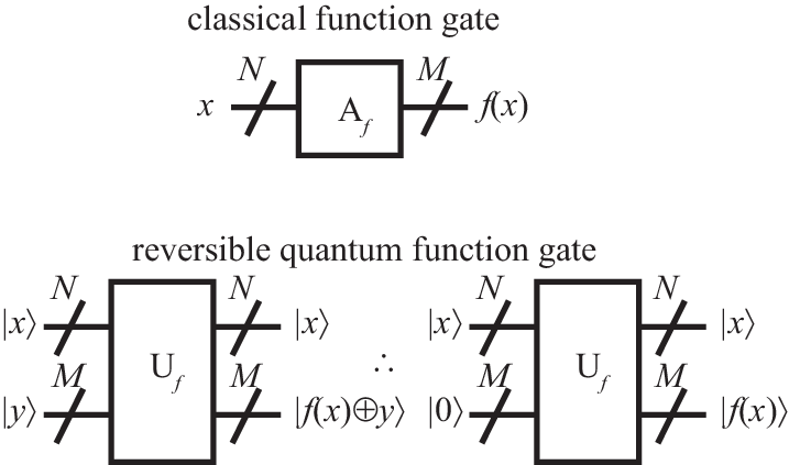
An important class of gates encountered in the following applications implement functions $f:x\to f(x)$, where $x$ is an $N$-bit input, and $f(x)$ is an $M$-bit output (see Fig. 7). In general, such functions are not invertible. The bottom panel of the figure shows a strategy to implement reversible versions of these functions: add auxiliary output channels which keep track of the input, and auxiliary input channels which when set to $0$ gives the desired outcome. (The auxiliary channels are called ancillas, and also feature prominently in error correction, section VI.1.) This can be achieved using the bit-wise XOR operation

	$f\oplus y$	$=$	$f_M\mathrm{\dots }{f}_1{f}_0\oplus y_M\mathrm{\dots }{y}_1{y}_0$
		$=$	$(f_M\oplus y_M)\mathrm{\dots }(f_1\oplus y_1)(f_0\oplus y_0).$

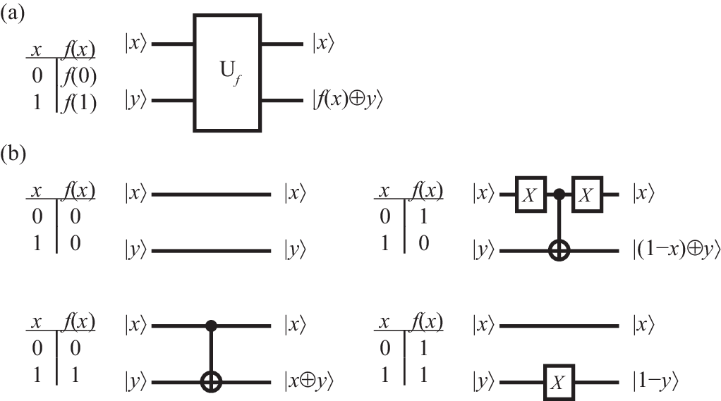
Functions with single-bit output are called Boolean functions (because their output can be interpreted as 0=FALSE, 1=TRUE). If the input $x$ is also only a single bit, there are exactly four function gates, which can be implemented in terms of elementary gates as shown in Fig. 8. If the auxiliary input state is set to $|y⟩=|0⟩$, they implement reversible versions of the four classical unary operators discussed in section II.5.