XV Angular momentum

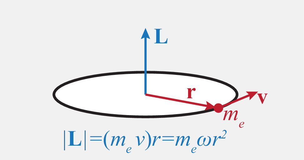
Classical angular momentum is given by

$$𝐋=𝐫\times 𝐩=(y{p}_z-z{p}_y)𝐢+(z{p}_x-x{p}_z)𝐣+(x{p}_y-y{p}_x)𝐤.$$

(259)

The angular momentum operator $\widehat{𝐋}=\widehat{𝐫}\times \widehat{𝐩}$ has components

	${\widehat{L}}_x=\widehat{y}{\widehat{p}}_z-\widehat{z}{\widehat{p}}_y=-i\mathrm{\hslash }(y{\displaystyle \frac{\partial }{\partial z}}-z{\displaystyle \frac{\partial }{\partial y}}),$		(260)
	${\widehat{L}}_y=\widehat{z}{\widehat{p}}_x-\widehat{x}{\widehat{p}}_z=-i\mathrm{\hslash }(z{\displaystyle \frac{\partial }{\partial x}}-x{\displaystyle \frac{\partial }{\partial z}}),$		(261)
	${\widehat{L}}_z=\widehat{x}{\widehat{p}}_y-\widehat{y}{\widehat{p}}_x=-i\mathrm{\hslash }(x{\displaystyle \frac{\partial }{\partial y}}-y{\displaystyle \frac{\partial }{\partial z}}).$		(262)

Total angular momentum is given by

$${\widehat{𝐋}}^2={\widehat{L}}_x^2+{\widehat{L}}_y^2+{\widehat{L}}_z^2=-{\mathrm{\hslash }}^2{\mathrm{\Delta }}_{\theta ,\varphi }.$$

(263)

The commutation relations are

	$[{\widehat{L}}_x,{\widehat{L}}_y]=i\mathrm{\hslash }{\widehat{L}}_z,[{\widehat{L}}_y,{\widehat{L}}_z]=i\mathrm{\hslash }{\widehat{L}}_x,[{\widehat{L}}_z,{\widehat{L}}_x]=i\mathrm{\hslash }{\widehat{L}}_y,$
			(264)
	$[{\widehat{L}}_x,{\widehat{𝐋}}^2]=0,[{\widehat{L}}_y,{\widehat{𝐋}}^2]=0,[{\widehat{L}}_z,{\widehat{𝐋}}^2]=0.$		(265)

Heisenberg’s uncertainty principle dictates that it is not possible to know two components of angular momentum at the same time (since their commutator does not vanish). However, it is possible to determine one of the components (say $L_z$) simultaneously with the total angular momentum, since $[{\widehat{L}}_z,{\widehat{𝐋}}^2]=0$.

We already determined that the spherical harmonics $Y_{lm}$ are joint eigenfunctions of ${\widehat{𝐋}}^2$ and ${\widehat{L}}_z$,

$${\widehat{𝐋}}^2{Y}_{lm}(\theta ,\varphi )={\mathrm{\hslash }}^{2}l(l+1)Y_{lm},$$

(266)

$${\widehat{L}}_z{Y}_{lm}(\theta ,\varphi )=\mathrm{\hslash }m{Y}_{lm}.$$

(267)

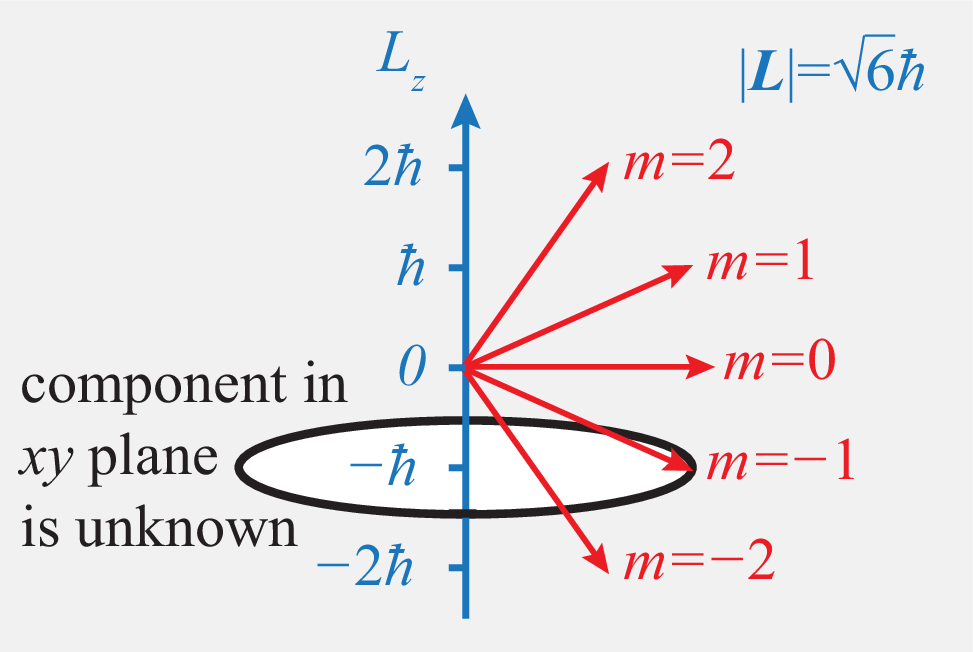
The eigenvalues are ${\mathrm{\hslash }}^{2}l(l+1)$ and $\mathrm{\hslash }m$, respectively. E.g., for $l=2$ the length of the angular momentum vector is $|𝐋|=\sqrt{6}\mathrm{\hslash }$ and there are 5 possible values values of $L_z$, as is illustrated in the following figure.

Instead of interpreting the angular Schrödinger equation as a differential equation, this equation can be solved very efficiently by employing the perspective of operators and vectors.

In Dirac notation, the eigenstates of the ${\widehat{L}}_z$ and ${\widehat{𝐋}}^2$ are denoted as $|lm⟩$, such that

$${\widehat{L}}_z|lm⟩=\mathrm{\hslash }m|lm⟩,{\widehat{𝐋}}^2|lm⟩={\mathrm{\hslash }}^{2}l(l+1)|lm⟩.$$

(268)

We now introduce the ladder operators ${\widehat{L}}_{\pm }={\widehat{L}}_x\pm i{\widehat{L}}_y$, which are non-hermitian and related by ${\widehat{L}}_{+}^{†}={\widehat{L}}_{-}$. These operators fulfill the commutation relation

$$[{\widehat{L}}_z,{\widehat{L}}_{\pm }]=[{\widehat{L}}_z,{\widehat{L}}_x]\pm i[{\widehat{L}}_z,{\widehat{L}}_y]=i\mathrm{\hslash }{\widehat{L}}_y\pm \mathrm{\hslash }{L}_x=\pm \mathrm{\hslash }{L}_{\pm }.$$

(269)

The utility of these operators arises from the fact that they relate the eigenstates $|lm⟩$ of fixed $l$ but different $m$ in a systematic way. Indeed, the following calculation shows that ${\widehat{L}}_{\pm }|lm⟩$ is still an eigenstate of $L_z$,

$${\widehat{L}}_z({\widehat{L}}_{\pm }|lm⟩)={\widehat{L}}_{\pm }{\widehat{L}}_z|lm⟩+[{\widehat{L}}_z,{\widehat{L}}_{\pm }]|lm⟩=\mathrm{\hslash }(m\pm 1){\widehat{L}}_{\pm }|lm⟩,$$

(270)

with eigenvalue $\mathrm{\hslash }(m\pm 1)$. Furthermore, because $[{\widehat{𝐋}}^2,{\widehat{L}}_{\pm }]=0$ this state is also an eigenstate of ${\widehat{𝐋}}^2$, with eigenvalue ${\mathrm{\hslash }}^{2}l(l+1)$. Thus,

$${\widehat{L}}_{\pm }|l,m⟩=c_{lm}^{\pm }|l,m\pm 1⟩,$$

(271)

where the normalisation constants work out as

$$c_{lm}^{+}=\mathrm{\hslash }\sqrt{(l-m)(l+m+1)},c_{lm}^{-}=c_{l,-m}^{+}.$$

(272)

Since $c_{ll}^{+}=0$, the state $|ll⟩$ is determined by the condition

$${\widehat{L}}_{+}|ll⟩=|\mathbb{𝟘}⟩,$$

(273)

while all other states follow by repeated application of ${\widehat{L}}_{-}$.

This construction of the angular momentum eigenstates and determination of their eigenvalues is purely algebraic, and sidesteps any explicit reference to spherical harmonics. Their explicit form can be recovered by writing $⟨\theta ,\varphi |lm⟩=Y_{lm}(\theta ,\varphi )$, where $|\theta ,\varphi ⟩$ denotes position basis states on the unit sphere, parameterised in spherical polar coordinates. $Y_{ll}$ is then obtained from Eq. (273), where ${\widehat{L}}_{+}$ is expressed as the associated differential operator, and the other spherical harmonics follow by successive application of the differential operator associated with ${\widehat{L}}_{-}$.

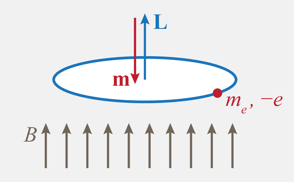
The orbital motion of an electron with angular momentum $𝐋$ gives rise to a magnetic moment

$$𝐦=-\frac{e}{2m_e}𝐋.$$

(274)

When a magnetic field $𝐁$ is applied, this gives rise to an interaction energy

$$V_B=-𝐦\cdot 𝐁,$$

(275)

which can be used to measure the angular momentum. We assume that the magnetic field is applied in $z$ direction, $𝐁=B_z𝐤$, therefore

$$V_B=\frac{e{B}_z}{2m_e}{L}_z.$$

(276)

Quantum mechanically the interaction energy is represented by the operator

$${\widehat{V}}_B=\frac{e{B}_z}{2m_e}{\widehat{L}}_z.$$

(277)

In a central potential a magnetic field hence lifts the $2l+1$ fold degeneracy of the angular part of the wavefunction: For each value of m, the energies of the orbitals are shifted by an amount

$$\delta E_m={\mu }_B{B}_{z}m,$$

(278)

which depends on the magnetic quantum number $m$ (hence the name). Here ${\mu }_B=\frac{e\mathrm{\hslash }}{2m_e}$ is the so-called Bohr magneton.