In my last two blog posts I focused on how to analyse the results of clinical trials through both Meta Analysis and Simultaneous Inference. Here we’re going to take a step back and look at how we choose a suitable model with relevant variables considered.
Directed Acyclic Graphs (DAGs) are used as a visual representation of associations between variables or factors in models. I first came across them in an Epidemiological context during the MATH464 course on Principles of Epidemiology given by Tom Palmer here at Lancaster University and thought I’d share the basic concepts with you all. Although I’ll discuss them in an epidemiology setting, DAGs can be used in a variety of applications to demonstrate associations and causal effects.
We’ll start with a simple definition of what DAGs are:
- Directed – all variables in the graph are connected by arrows.
- Acyclic – if we start at a variable X, following the path of the arrows we shouldn’t be able to get back to X.
- Graph – we have nodes which represent factors/variables and arrows that represent causal effects of one factor on another.
Another useful definition is that of a path: a path is any consecutive sequence of arrows regardless of their direction. A backdoor path is where we start a path by moving in the wrong direction down an arrow.
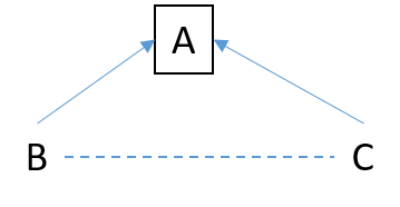
The idea of a DAG is best illustrated through an example. The following example was outlined by Williams et. al (2018) in which the factors affecting obesity in children were considered:
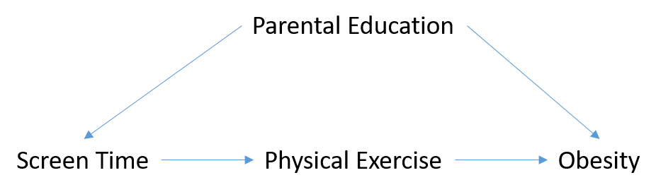
This DAG suggests that a low parental education may increase the amount of screen time a child is engaging in, hence reducing their level of physical exercise. This in turn will increase their risk of obesity. Parental education is also a cause of obesity, hence, parental education is a common cause of both increased screen time and obesity. This is what we call a confounder variable which we’ll return to later.
We say that any two variables are d-connected if there is an unblocked path between two variables, this usually implies they are dependent on one another.
Within DAGs we have several types of variables, all of which need to be handled in different ways when considering how to analyse a model:
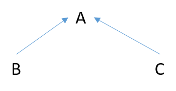
- Collider – a node where two arrows meet.
- Confounder – Pearl’s (2009) definition of confounding is the existence of an open backdoor path between two variables X and Y.
- Mediator – an intermediate variable that lies on the causal pathway between two variables.
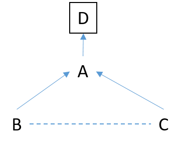
If we extend the previous example to include self-esteem in the model:
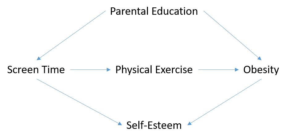
In this example, self-esteem is a collider as both obesity and increased screen time reduce self-esteem. Physical exercise is a mediator between screen time and obesity as it lies on the causal pathway. Finally, parental education is a confounder as it both increases screen time and obesity and hence creates a backdoor path between the two.
Now we have constructed a DAG, how do we use this to create a statistical model? We use the following rules to decide which variables to control for. We can control for a variable in several ways including conditioning on a variable by using the variable as a covariate in the regression model, stratifying by the variable or using matching techniques in trial recruitment.
D-seperation Rules (Palmer, 2018):
- If no variables are conditioned on, a path is blocked if and only if there is a collider located somewhere on the pathway between exposure and outcome.
- Conditioning on a confounder blocks the path.
- If we condition on a collider it doesn’t block the path, in fact, it creates a path between exposure and control. This may mask the true relationship between two variables or indicate a relationship when none in fact exists. This is known as collider bias.
- Also, a collider that has a descendant that has been conditioned on doesn’t block the path.
If we control for a confounder we reduce bias but if we adjust for a collider we increase bias. Collider bias is responsible for many cases of bias in modelling and is often not dealt with properly (Barrett, M. (2020)). This is what makes DAGs such a useful tool in modelling. It gives a visual representation of how things are associated with one another and can indicate where bias is being induced in models.
Modelling through DAGs may be easy for simple situations with only a few variables but it gets very complicated very quickly when the number of variables and associations increases.
For further reading, I would recommend the paper by Evandt et. al (2018) in which they use DAGs to model the association between road traffic noise and sleep disturbances by considering variables such as socioeconomic status and lifestyle. However, to see how DAGs are applied outside of an epidemiological setting I would recommend the paper by Al-Hawri et. al (2019), where they use DAGs to model wireless sensor networks.
I hope you enjoyed this blog post on DAGs!
References
- Al-Hawri, E., Correia, N., Barradas, A., (2020). DAG-Coder: Directed Acyclic Graph-Based Network Coding for Reliable Wireless Sensor Netowrks. IEEE Access 8.
- Barrett, M., (2020). An Introduction to Directed Acyclic Graphs. Cran R Project: https://cran.r-project.org/web/packages/ggdag/vignettes/intro-to-dags.html
- Evandt, J., Oftedal, B., Hjertager Krog, N., Nafstad, P., Schwarze, P., Marit Aasvang, G., (2016). A population-based study on nighttime road traffic noise and insomnia. SLEEP, 40(2).
- Palmer, T., (2018). Principles of Epidemiology MATH464 Lecture Notes. Lancaster University.
- Pearl, J., (2009). Causality: Models, Reasoning and Inference. Cambridge University Press 2nd Edition.
- Sttorp, M., Siegerink, B., Jager, K., Zoccali, C., Deker, F., (2015). Graphical Presentation of Confounding in Directed Acyclic Graphs. Nephrology Dialysis Transplantation, 30(9).
- Williams, T., Bach, C., Mattiesen, N., Henriksen, T., Gagliardi, L., (2018). Directed Acyclic Graphs: A Tool for Causal Studies in Pediatrics. Pediatric Research, 84(4).