The Travelling Salesman Problem (TSP) is a classic optimization problem within the field of operations research. It was first studied during the 1930s by several applied mathematicians and is one of the most intensively studied problems in OR.
The TSP describes a scenario where a salesman is required to travel between \(n\) cities. He wishes to travel to all locations exactly once and he must finish at his starting point. The order in which the cities are visited is not important but he wishes to minimize the distance traveled. This problem can be describes as a network, where the cities are represented by nodes which are connected by edges that carry a weight describing the time or distance it takes to travel between cities.
This problem may sounds simple and using a brute force method in theory it is: calculate the time to transverse all possible routes and select the shortest. However, this is extremely time consuming and as the number of cities grows, brute force quickly becomes an infeasible method. A TSP with just 10 cities has 9! or 362,880 possible routes, far too many for any computer to handle in a reasonable time. The TSP is an NP-hard problem and so there is no polynomial-time algorithm that is known to efficiently solve every travelling salesman problem.
Because of how difficult the problem is to solve optimally we often look to heuristics or approximate methods for the TSP to improve speed in finding the solution and closeness to the optimal solution.
The TSP can be divided into two types: the asymmetric travelling salesman problem (ASTP) where the distance from A to B is different to that from B to A and the symmetric travelling salesman problem (STSP) where the distance from A to B is the same as from B to A. For example, the ASTP may arise in cities such as Lancaster where there are one-way roads that make travelling more varied. In this blog I will be focusing on the STSP and outline two of the most basic heuristic algorithms in which to solve them.
Nearest Neighbor Algorithm
One of the simplest algorithms for approximately solving the STSP is the nearest neighbor method, where the salesman always visits the nearest city. The process is as follows:
- Select a starting city.
- Find the nearest city to your current one and go there.
- If there are still cities not yet visited, repeat step 2. Else, return to the starting city.
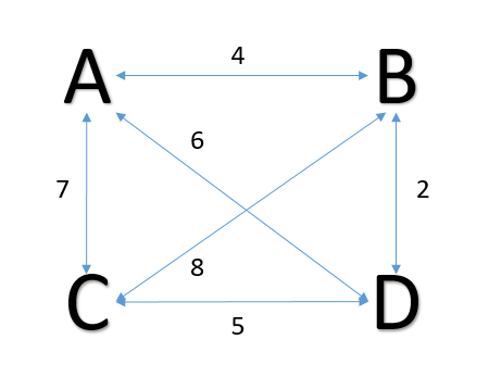
Using the nearest neighbor algorithm on the below symmetric travelling salesman problem starting at city A, we would then travel to city B followed by D and C, returning back to A. This gives a total length of 18, which in this case is indeed optimal. However, the nearest neighbor algorithm does not always achieve optimality.
For example if we change the weight slightly:
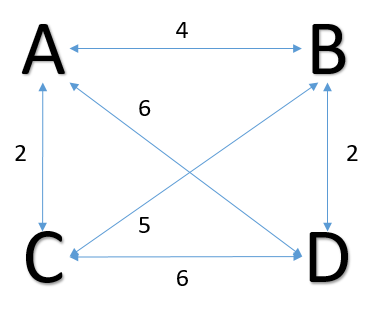
The solution using the nearest neighbor algorithm starting again at A will result in the Route A -> C -> B -> D -> A, resulting in a route of weight 15. But this is not optimal. If we instead took the route A -> B -> D -> C -> A the weight would be 14, a slight improvement on that obtained by the algorithm. Therefore the algorithm achieved a sub-optimal result.
This algorithm under worst-case performance is \(\mathcal{O}(n^2)\), much better than the brute force method (which is \(\mathcal{O}(n!)\)). It is easy to implement but the greediness of the algorithm does cause it to run quite a high risk of not obtaining the optimal route.
Greedy Approach Algorithm
Before we delve into the next algorithm to tackle the TSP we need the definition of a cycle. A cylce in a network is defined as a closed path between cities in which no city is visited more than once apart from the start and end city. The order of a node or city is the number of edges coming in or out of it.
The greedy algorithm goes as follows:
- Sort all of the edges in the network.
- Select the shortest edge and add it to our tour if it does not violate any of the following conditions: there are no cycles in our tour with less than \(n\) edges or increase the degree of any node (city) to more than 2.
- If we have \(n\) edges in our tour stop, if not repeat step 2.
Applying this algorithm to the STSP in Figure 1, we begin by sorting the edge lengths:
B <-> D = 2, A <-> B = 4, C <-> D =5, A <-> D =6, A <-> C =7, C <-> B =8
We then add the routes B <-> D, A <-> B and C <-> D to our tour without problem. We cannot add A <-> D to our tour as it would create a cycle between the nodes A, B and D and increase the order of node D to 3. We therefore skip this edge and ultimately add edge A <-> C to the tour. This results in the same solution as obtained by the nearest neighbor algorithm.
If we then apply the method to the STSP given in Figure 2 we obtain the optimal route: A -> B -> C -> D -> A. This is an improvement on what was achieved by the nearest neighbor algorithm.
This algorithm is \(\mathcal{O}(n^2\log_2(n))\), higher than that of the nearest neighbor algorithm with only a small improvement in optimality.
References and Further Reading
As said above, these are only two of the most basic algorithms used to obtain an approximate solution to the travelling salesman problem and there are many more sophisticated methods. If you wish to read more about these, I would suggest reading the following two papers:
- Nilsson, C., (2003). Heuristics for the Traveling Salesman Problem. Linkoping University. Link.
- Abdulkarim, H., Alshammari, I., (2015). Comparison of Algorithms for Solving Traveling Salesman Problem. International Journal of Engineering and Advanced Technology 4(6).