
In a recent talk given to the MRes students, I was asked for my opinion on a multi-armed bandit problem. In these working from home times, I’m sure most of us know of the combined dread and panic that comes with taking your microphone off mute to speak on a call. I contemplated the question, and then gave my answer. As you might have guessed from the title of this talk, I was wrong. But I certainly wouldn’t get this problem wrong again, because I had learned from my mistake.
Ironically enough, learning from your mistakes, or past behaviour, is an idea that is strongly rooted in the multi-armed bandit problem. And thus, a blog post was inspired!
Multi-armed bandits
So, let’s get started. What exactly is a multi-armed bandit?
When most people hear ‘multi-armed bandit’, they may think of gambling. That is because a one-armed bandit is a machine where you can pull a lever, with the hopes of winning a prize. But of course, you may not win anything at all. It is this idea which constitutes a multi-armed bandit problem.
Mutli-armed bandit problems are a class of problems where we can associate a particular score with each of our decisions at each point in time. This score includes the immediate benefit or cost of making that decision, plus some future benefit.
Imagine that we have K independent one-armed bandits, and we get to play one of these bandits at each time t = 0, 1, 2, 3, …. These are very simple bandits, where we either win or lose upon pulling the arm. We’ll define losing as simply winning nothing.
Now, if your win occurs at some time t, then you gain some discounted reward at, where 0 < a < 1. Clearly, rewards are discounted over time; this means that a reward in the future is worth less to you than a reward now. The mathematically minded among you may realise that this means that the total reward we could possibly earn is bounded.
The probability of a success upon pulling bandit i is unknown, and denoted by πi. Since these success probabilities are unknown, we have to learn about what the πis are and profit from them as we go. This means that, in the early stages we have to pull some of the arms just to see what πi might be like.
At each time t, our choice of which bandit to play is informed by each bandit’s record of successes and failures to date. For example, if I know that bandit 2 has given me a success every time I pulled it, I might be inclined to pull bandit 2 again. On the other hand, if bandit 4 has given me a failure most of the times, I might want to avoid this bandit. Thus, we are using previous data which we have obtained about each of the bandits in order to update our beliefs about the bandits’ probability distributions.
The Maths
Updating our beliefs about the probability distributions of the bandits in this way is using an interpretation of statistics called Bayesian. Let’s imagine that we have a parameter that we want to determine (in our case, the probability of success for each of the K bandits). Maybe we have some prior ideas about what the probability of success for each bandit will be. This could be due to previous experiments you know about, or maybe just personal beliefs. These prior beliefs are described by the prior distributions for the parameters.
Then, let’s imagine we begin our bandit experiment. After time t, we have pulled t bandits, and we now have information detailing the number of successes and failures for each of the bandits pulled. At this time, we take this observed data into account in order to modify what we think the probability distributions for the parameters look like. These updated distributions are called the posterior distributions.
The Question…
How do we play the one-armed bandits in order to maximise the total gain?
Well, this is where the importance of learning from your mistakes comes in. Imagine the case where K = 5, and at time t = 7 our observed data are as follows:
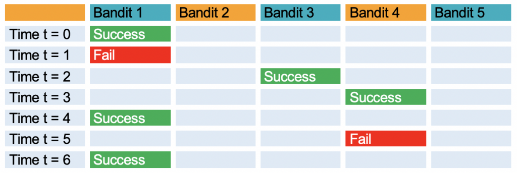
Looking at our observed data, bandit 1 has the highest proportion of successes out of the number of times it was played. So maybe we would want to pull Bandit 1 again at our next time?
Well, maybe not.
Notice that Bandits 2 and 5 haven’t been played yet at all; therefore we can’t really infer any data about them. Pulling Bandit 1 might give us a success on our next attempt, but it could also give us a fail. We know nothing about Bandits 2 and 5, perhaps these bandits have a probability of success of 1?
The idea of pulling the best bandits to maximise your expected number of successes relies on a balance between exploration and exploitation. Exploration refers to playing bandits that we don’t know much about, in this case, pulling arms 2 and 5. Exploitation, on the other hand, means pulling the arms of bandits that we already know might give us a good result; in our case, pulling bandit 1 again.
Every time we pull an arm, we are actually receiving both a present benefit and a future benefit. The present benefit is what we win, and the future benefit is what we learn. Recall that at time t, if we win, we receive a discounted reward of at. Therefore, the closer a is to 1 determines how important it is to learn about the future. For example, if a is closer to one, many future pulls will make a big difference. On the other hand, if a is closer to 0, our present benefit is more important. Again, this relates to the importance of balancing exploration and exploitation.
So how do we quantify both the immediate benefit and the future benefit from these bandits, in such a way so that we can play the bandits to maximise our total gain? It is possible to take the posterior distribution for each bandit at each point in time, and associate a score with it that represents both future and present benefit of pulling that bandit.
It turns out that there is something called a Gittins Index, which is a value that can be assigned to every bandit. By looking at the Gittins Index for all K bandits at time t, it is Bayes optimal to play any bandit which has the largest Gittins index, which is pretty cool!
So there we have it, learning from past experiences is critical in the world of multi-armed bandits, and also in many other areas of mathematics including reinforcement learning and bayesian optimisation. The trade off between exploration and exploitation is critical, and perhaps even serves as a reminder to the importance of not being afraid to make mistakes in our everyday lives… just a thought.
If you enjoyed this post, be sure to check out the following further reading resources!
Further Reading
Introduction to Multi-Armed Bandits – Aleksandrs Slivkins This book gives a good introduction to multi-armed bandits for those interested, and goes into detail on some of their many uses.
These lecture notes are really great for those of you looking for a gentle introduction to the Gittins index and multi-armed bandits! Those new to the subject may also want to look at the Wikipedia page as a good starting point.
Multi-Armed Bandits and the Gittins Index – P. Whittle.
If you’re interested in exploration vs exploitation in reinforcement learning, check out this post and this post.
If you’re interested in exploration vs exploitation in Bayesian optimisation, check out this post.