MCMCMC

Over Christmas I was set the task of writing a report about something that interested my during my first term of the MRes. I chose to look into something called Metropolis-Coupled Markov Chain Monte Carlo (MCMCMC). This sounds like a mouthful but once broken down isn’t too scary.

I will start off by giving a brief explanation of what Markov Chain Monte Carlo (MCMC) is. Imagine you have a probability density function \( \pi(x) \) and you need to take random samples from it, but your function is too complicated to work this out by hand. What MCMC does is find a way to simulate taking random draws by constructing a random walk that moves by taking into account this complicated function. The simplest way to do this is called Random Walk Metropolis (RWM).

We start off with some initial position \( x \). Then we propose a new position by adding a normal sample to it \( y = x + \mathcal{N}(0, h) \) where \(h\) is something the user can tune. There is then a Metropolis-Hastings acceptance step where we try to determine if \(y\) is a sensible sample for our distribution to take. To do this we let \( A = \min \left( 1, \frac{\pi(y)}{\pi(x)} \right) \) and then accept \( y \) as our new position with probability \( A \). This is then repeated to get as many samples as you wish.

Of course the downside of such a simple method is that it will only work in certain cases. Having a multi-modal distribution is something that makes RWM perform very badly. What I mean by perform badly is that we get very dependent samples which is not desirable if we would like to use them for any kind of analysis about the distribution.

This motivates the need for more complicated methods, and one that works well in this scenario is MCMCMC. What we now do is we take multiple probability density functions \( \pi_1(x), \pi_2(x), \dots, \pi_m(x) \) and run RWM on each of these separately. We pick \( \pi_1(x) = \pi(x) \) and then for each other distribution we would like to ‘smooth out’ the function.

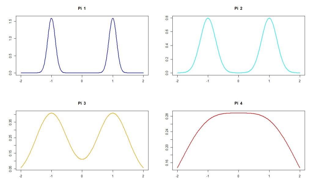
The clever part though is that after each iteration we introduce a Metropolis-Hastings step that can switch the position between any two of the chains. This allows us to get better movement with our random walk on \( \pi(x) \) as I will show from the results I obtained:

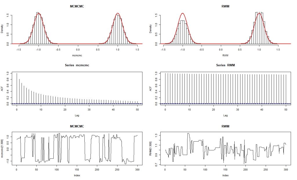
The top graphs show a histogram of the simulated results with the true distribution in red over the top. From this we can see that we’re getting a much better representation with MCMCMC. The second graphs show what is called an ACF plot and is used to measure the correlation of the data with a lagged version of the data. We wish this to converge to 0 since then we will be getting what appear to be independent results, and MCMCMC is getting much closer than RWM. The last graphs show the random walk for the first 300 steps. What we see is that MCMCMC is moving between the two peaks whereas RWM gets stuck in the the right peak.

If you would like to read more about this you can read my Christmas report here:

And if you would like to discuss MCMCMC or any other blog on my website please feel free to contact myself using the form below.