I recently finished a report on Bayesian nonparametrics and I figured a post to motivate the excitement around the area would be warranted. Since most of what goes on under the hood when modelling your problem this way is some pretty involved pure mathematics, let’s start with a concrete-ish problem. Here goes.
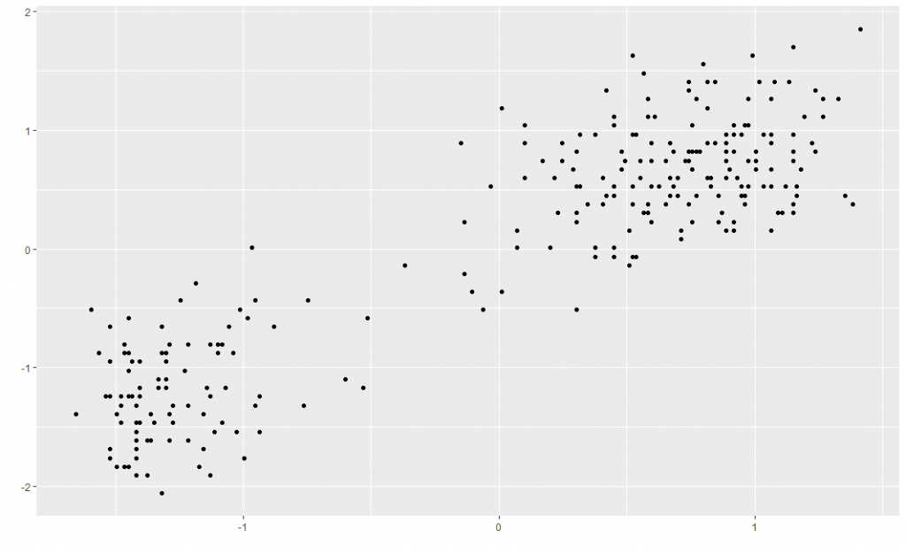
Say you want to cluster some data — group your observations in a meaningful way, without knowing anything about the groups beforehand. A classic example is the Old Faithful dataset built into R, which has 272 observations of eruption duration and waiting time between eruptions for the eponymous geyser in the Yellowstone national park. This is what the centred and scaled dataset looks like — there are two clear groups which you’d hope your clustering method would pick up.
The default statistical way to go about clustering is to assume the data comes from a finite mixture distribution
p(x ; \bm\theta ) = \sum_{i=1}^{K} \pi_i p(x ; \theta_i ),where each mixture component corresponds to a group. You could then get parameter estimates (for pi and theta) using the expectation-maximization algorithm. You have to specify how many groups there are before even doing your estimation though, which seems counter-intuitive. The workaround is to do this for several models, each with a different number of groups K, and pick the best fitting model by some criterion.
But what if you didn’t have to do any workaround? The Bayesian nonparametric approach comes to the rescue. Introducing… the Dirichlet process (DP), a stochastic process whose draws are probability distributions. The idea is to have a single model, which uses the DP as a prior: conceptually speaking, a probability distribution is sampled from the DP then a parameter is sampled from that distribution. To write the model out, this is
\begin{aligned} H &\sim \text{DP}(a,G)\\ \theta_i | H &\sim H\\ x_i | \theta_i &\sim p(x ; \theta_i ), \end{aligned}where the scalar a determines how strongly clustered the observations tend to be and and the probability distribution G determines the location of the cluster parameters. Together, they fully specify the DP.
The reason why this model makes sense is that the DP has a natural clustering property. Forgetting about the likelihood for the moment, assume we’ve clustered n observations already. Introducing an extra observation and integrating out the DP, the predictive distribution for its parameter is
\theta_{n+1} | \theta_1,\dots,\theta_n \sim \frac{1}{n+a}\delta_{\theta_1}+\dots+\frac{1}{n+a}\delta_{\theta_n}+\frac{a}{n+a}G.In words, the new parameter takes the value of any one of the previous parameters with probability 1/(n+a), or a new parameter is generated from the distribution G with probability a/(n+a). What this amounts to is that observations clump together, with the strength of the clustering being specified by a — the larger it is, the more clusters there are.
Together with the likelihood, the hope is that this natural clustering property encourages observations to fall in the “right” clusters. More satisfyingly, the number of clusters is set automatically, so there is no need to select it by model comparison.
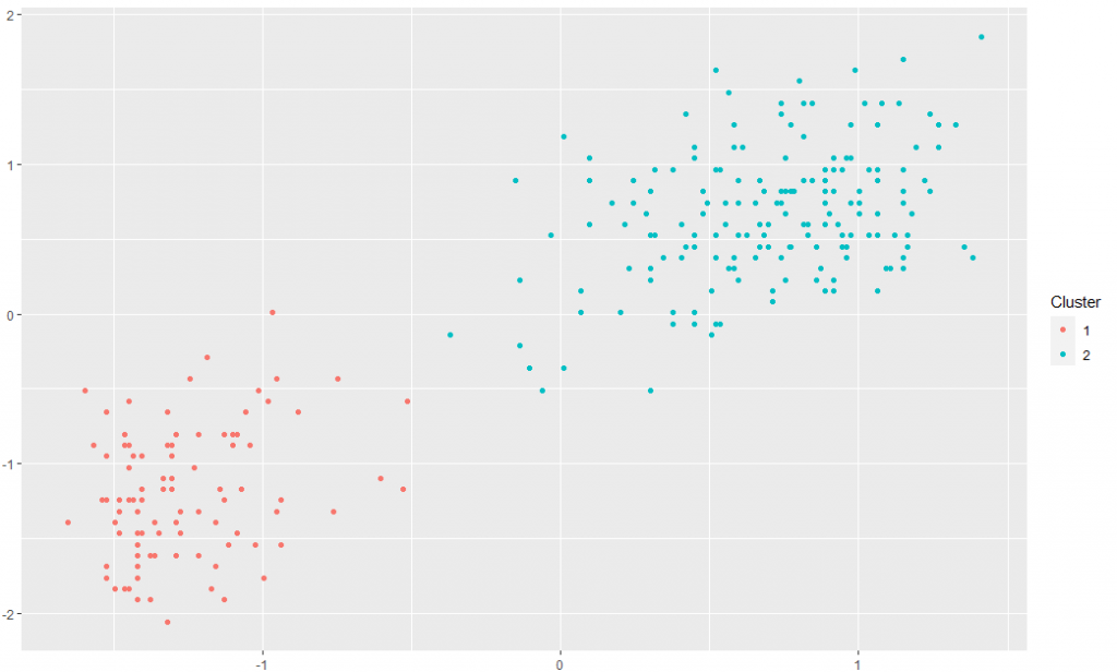
And it actually works. I’ve run the DP clustering model on the Old Faithful dataset using the “dirichletprocess” R package with default parameters. After 1000 MCMC iterations, the clusters look like you would expect.
Further reading
[1] A collection of resources on Bayesian nonparametrics from Peter Orbanz
[2] These lecture notes from Leiden University are a good introduction to the finer mathematical points
[3] dirichletprocess CRAN page

Thanks for the clear explanation!