
1. Introduction
Around the world, mining disasters are the source of thousands of deaths every year. Amongst the different types of mining methods, underground coal mining is particularly dangerous. This was especially true during the 19th century and led to the creation of the Coal Mines Regulations Act of 1887, which took effect in the United Kingdom on the 1st January 1888. Until then, it was not required to have ventilation in the mines and explosives could be stored underground, additionally, this act raised the minimal age for mine workers from 10 to 12 years old (note that until the 1840s, children as young as 5 years old took part in the industrial workforce) (Tailor, 1968). Social science researchers may be interested in finding out if such regulations have had an impact on the yearly number of mining disasters. This can contribute to a better understanding of what causes mining disasters and thus help further reduce them.
The data used for this project comes from the Colliery Year Book and Coal Trades Directory available from the National Coal Board in London (Jarrett, 1979). This data contains the count of annual coal mining disasters in the UK between 1851 and 1962. The aim of this project is to detect changes in the rate of yearly coal mining disasters in the UK between 1851 and 1962 using a Bayesian approach. We are not attempting to explain why the rates have changed but simply to identify if and when they may have happened. To do so, the method used in this project is known as Bayesian changepoint detection. Using this method, models with different number of changepoints were fitted to the data. To keep the blog clear, the model for three changepoints will often be used as an example. An additional goal was to determine the model which best explains the observed data. Fitting these models required the implementation of a sampling technique; for this project we used Direct Sampling. Direct Sampling was chosen as it does not rely on convergence unlike Markov Chain Monte Carlo methods.
2. Results
2.1 The Concept of Changepoint Detection for Mining Disasters
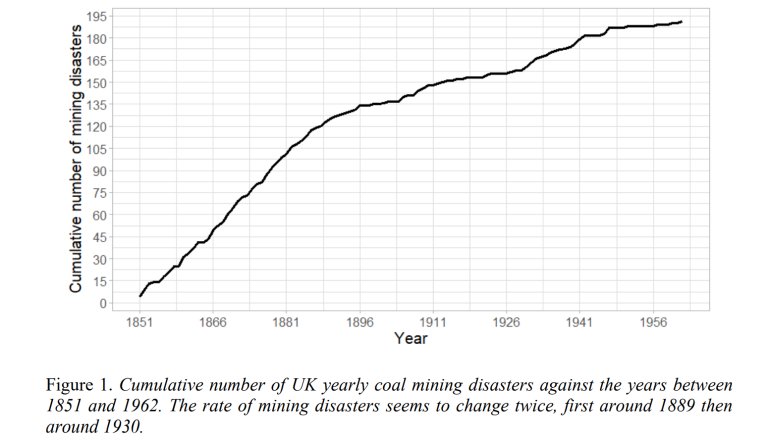
Let us assume a certain event occurs exactly the same number of times every year. When plotting the cumulative number of times this event occurs against the years, we would expect to observe a straight line. The cumulative number of UK coal mining disasters between 1851 and 1962 is displayed in Figure 1. The line in this plot is not straight, hence it seems that the number of yearly coal mining disasters is not constant between 1851 and 1962. Empirically, the rate of mining disasters appears to slow down just before the beginning of the 20th century.
We refer to a changepoint as the moment in time when the rate of an event occurring changes. In the context of this project, if we assume 𝑛 changepoints exist, then we denote 𝑇𝑘 as the date of the 𝑘𝑡ℎ changepoint (for 𝑘 = 1, 2, … , 𝑛). To simplify our calculations, time was recorded as a discrete variable, thus, although this is not exact, we have assumed a changepoint can only be located directly after the beginning of a year. Additionally, we presume the rate does not change in the first year and doing so limits 𝑇𝑘 to all integer values between 1852 and 1962. Therefore, when 𝑛 changepoints exist, the time series of the mining disasters is split into 𝑛 + 1 segments.
2.2 Identifying Most Likely Locations of Changepoints
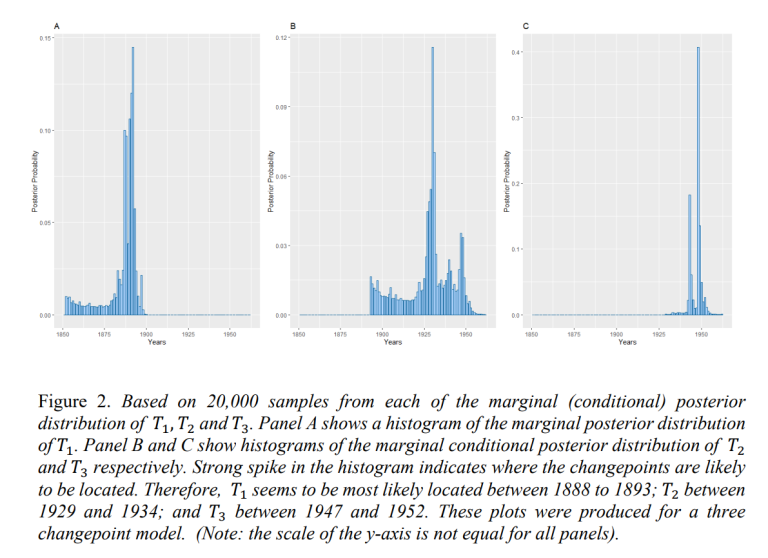
The first aim of this project was to identify where the changepoints are likely to have happen. This was done by calculating the corresponding marginal (conditional) posterior distribution. Figure 2 shows the marginal (conditional) posterior distribution of changepoints 𝑇1, 𝑇2, 𝑇3, obtained when using a three changepoint model. To detect where these changepoints are likely to have happened, 20,000 samples were taken from each marginal (conditional) posterior distribution. The mode of each 20,000 samples was taken to be the most likely location for the corresponding changepoint. The modes of 𝑇1, 𝑇2, 𝑇3, indicated that these are most likely located in 1892, 1930, 1948, respectively.
2.3 Identifying Coal Mining Disaster Rates
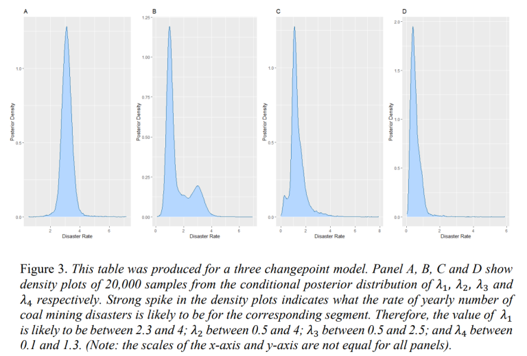
Using the samples of changepoint locations, it is now possible to sample the corresponding mining disaster rates. The mining disaster rates were sampled from their corresponding conditional posterior distribution. When choosing a model with 𝑛 changepoints, 20,000 samples were produced for each of the 𝑛 + 1 corresponding mining disaster rates. Figure 3 shows the conditional posterior distributions of 𝜆1, 𝜆2, 𝜆3 and 𝜆4. This helps us identify the rate of yearly mining disasters for each segment.
2.4 Predictions of the Cumulative Number of Coal Mining Disasters
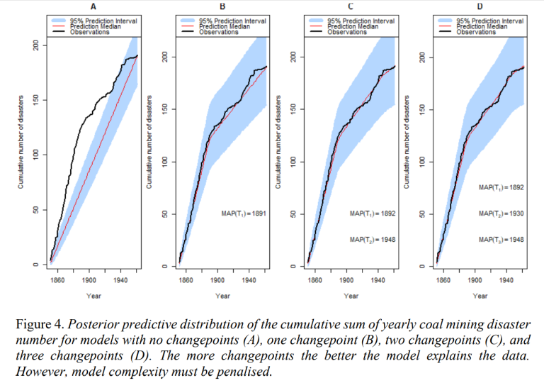
Using the data from the samples, we are now interested in producing predictions of the cumulative number of mining disasters. This was done using the 20,000 sampled location for each 𝑛 changepoints and 20,000 samples of each corresponding 𝑛 + 1 mining disaster rates. The median and 95% prediction interval of cumulative number of mining disasters for each year were computed. These give us the posterior predictive distributions of cumulative number of coal mining disaster; these are plotted in Figure 4.
These plots give us an idea of how well the models with different number of changepoints explain the data observed. From the models compared in Figure 4, three changepoints seems to best explain the data. However, this is expected, as the more changepoints we add, the more flexibility the models have to explain the data observed. However, to determine which model
best explains the data we will penalise the models’ complexity.
2.5 Model Selection
The third and final aim of this project was to compare models with different number of changepoints using marginal likelihood evaluation procedures. Occam’s razor tells us to favour the simpler models over more complex ones. Furthermore, Occam’s razor is a consequence of Bayesian inference (Jefferys & Berger, 1992). In the context of this project, it means that as more complex models (more changepoints) tend to be more flexible, that flexibility is automatically penalised by Bayesian inference. The marginal likelihood of a model with different number of changepoints were evaluated using equation 9; Figure 5 shows the results.
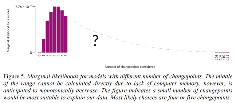
For more than seven changepoints, the models’ complexity meant that the marginal likelihoods could not be computed due to a lack of computer memory. However, the marginal likelihoods are expected to monotonically decrease, because the penalisation due to the addition of an extra changepoint outweighs the increase in how well the model explains the data. From Figure 5, we can see that four or five changepoints are most likely to best describe the observed data. The marginal likelihood of the model with four changepoints is very slightly greater, therefore, it can be considered as the best model to describe the data. When using a four changepoint model, the locations of changepoints are likely to be 1892, 1897, 1930 and 1948 for 𝑇1, 𝑇2, 𝑇3 and 𝑇4, respectively.
3. Conclusion
The aim of this project was to detect changes in the rate of yearly coal mining disasters in the UK between 1851 and 1962 using a Bayesian approach. Additionally, the goal was to determine the model which best explains the data observed. Direct sampling was chosen as the inference method implemented to fit models with different number of changepoints. The first step was to identify the most likely location for each changepoint by sampling from their respective marginal (conditional) posterior distribution. Then, their corresponding mining disaster rates were sampled from their conditional posterior distributions. With samples of both changepoint locations and mining disaster rates, samples of predicted yearly number of coal mining disasters were produced. These were then cumulatively summed before obtaining the corresponding posterior predictive distribution. To determine the model which best describes the observed data, marginal likelihood evaluation procedures were implemented. Because we used Bayesian inference, the models’ complexity was automatically penalised. Thus, we do not have to worry about models explaining the data well simply because they have many changepoints. Comparing the models revealed that a four changepoint model is most suitable to explain the data. These changepoints are most likely to be in 1892, 1897, 1930 and 1948 for 𝑇1, 𝑇2, 𝑇3 and 𝑇4, respectively