In the world of data analysis, detecting changes in data streams is a crucial task. This article will guide you through performing online (or real-time) changepoint detection using the focus-cpt Python package, to identify abrupt shifts in your data streams as quickly as they arrive.

Changepoint detection is a statistical technique used to pinpoint moments in a time series where the underlying characteristics of the data significantly change, such as a change in the mean, variance, or distribution of the data. This can be invaluable in various applications, from monitoring financial markets for sudden price fluctuations to tracking sensor readings for equipment failures.

Online changepoint detection, in particular, is useful when dealing with large datasets or real-time data streams. It allows us to detect changes in the data as they occur, rather than waiting until the end of the dataset, and this can be particularly useful in monitoring applications where timely detection is critical.

The focus-cpt package implements the FOCuS family of algorithms on top of an efficient C++ backend. These algorithms compute the Generalised Likelihood Ratio test for a single changepoint exactly, with a per-iteration cost of roughly O(log(n)) in the univariate case, making them ideal for processing large data streams efficiently, even with few (or no) training observations. The package supports various univariate and multivariate distribution families, including Gaussian, Poisson, Gamma, and Bernoulli. It can handle scenarios where the pre-change parameter is known or unknown, one-sided and two-sided alternatives, non-parametric detection, and even data streams with autocorrelated noise.

If you prefer working in R, check out the companion guide: How to Perform Online Changepoint Detection in R. The two packages share the same interface and produce the same results.

If you have found the focus-cpt package useful, or encountered any limitations or issues, please get in touch – we would love to hear from you!

Getting Started

The focus-cpt package is readily available through PyPI:

pip install focus-cpt

Alternatively, the development version can be installed from the GitHub repository:

pip install "git+https://github.com/gtromano/unified_focus.git#subdirectory=focus_cpt"

Note that, while the package is called focus-cpt, the module is imported as focus_cpt (with an underscore).

Detecting a Change in Mean for Univariate Gaussian Distribution

As a first example, here, we’ll demonstrate how to detect a change in mean for a univariate Gaussian distribution. We’ll simulate some data with a shift in mean at a specific point and then use the package to pinpoint this changepoint.

Simulating the Data

First, we’ll import the necessary libraries and generate some sample data that embodies a change in mean.

import matplotlib.pyplot as plt
import numpy as np

# Set random seed for replicability
np.random.seed(0)

# Define data means and sizes
mean_pre = 0.0
mean_post = 2.0
size_total = 50000  # Total data size

# Generate data with a changepoint in the middle
Y = np.concatenate((np.random.normal(loc=mean_pre, scale=1.0, size=int(size_total / 2)),
                    np.random.normal(loc=mean_post, scale=1.0, size=int(size_total / 2))))

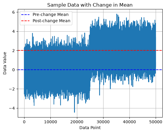
To generate the example in this snippet, we define the means (pre-change and post-change) and the total data size (size_total), and define the pre-change and post-change segments by dividing the total size in half. This generates a changepoint in the middle, as it can be seen in the plot below:

# Plot the data to visualize the changepoint
plt.plot(Y)
plt.axhline(y=mean_pre, color='b', linestyle='--', label='Pre-change Mean')
plt.axhline(y=mean_post, color='r', linestyle='--', label='Post-change Mean')
plt.xlabel('Data Point')
plt.ylabel('Data Value')
plt.title('Sample Data with Change in Mean')
plt.legend()
plt.grid(True)
plt.show()

Online Changepoint Detection

Time to run our changepoint analysis! In real-world monitoring scenarios, data typically arrives as a stream. The focus-cpt package is designed for this type of online or real-time analysis. Imagine the data is continuously fed into a buffer, and the changepoint detection algorithm analyzes this buffer to identify potential shifts in the underlying distribution.

For the sake of this article, we simulate this process by iterating over the data points one by one. In a streaming application, the loop would be replaced by a mechanism to pull data from the buffer whenever new data arrives.

from focus_cpt import Detector

detector = Detector(type="univariate")
threshold = 25.0

for y in Y:
    # Sequentially update the detector with each data point
    detector.update(y)
    result = detector.get_statistics(family="gaussian")
    if result["stat"] >= threshold:
        break

print(f"Change detected at time {result['stopping_time']:.0f}, "
      f"changepoint estimated at {result['changepoint']:.0f}")

Change detected at time 25004, changepoint estimated at 25000

After 25,000 data points, we detected our changepoint only after 4 iterations!

Explanation:

• We create a detector object with Detector(type="univariate") and we set a threshold (threshold = 25.0) for the detection statistic. In this example we go with a fixed threshold, however this can be tailored to each application’s needs.

The core loop iterates through the data (Y), mimicking how the detector would process a stream of data points arriving one at a time:

• Inside the loop, each data point y is fed to the detector using detector.update(y). This function internally updates the detector’s candidate changepoints to track the evolving data stream.

• The detector.get_statistics(family="gaussian") call computes the current value of the detection statistic — a likelihood ratio statistic quantifying how likely a change has occurred based on the data seen so far. Note how the distribution family is specified here, at query time, and not when the detector is created: the state of the detector is independent of the statistic computed on it (more on this later).

• If the detection statistic surpasses the predefined threshold, it suggests a significant shift in the data stream is probable. We break out of the loop and assume a changepoint has been detected.

• The result is a dictionary reporting the stopping_time (when we detected the change), the estimated changepoint location, and the value of the test statistic stat.

Offline Mode

If the data is already sitting in memory — say, for a retrospective analysis, or for calibrating a threshold on some training data — the focus_offline function runs the very same analysis with the whole loop executed in C++, which is considerably faster:

from focus_cpt import focus_offline

res = focus_offline(Y, threshold=25.0, type="univariate", family="gaussian")
print("Detection time:", int(res["detection_time"]))
print("Estimated changepoint:", int(res["detected_changepoint"]))

Detection time: 25004
Estimated changepoint: 25000

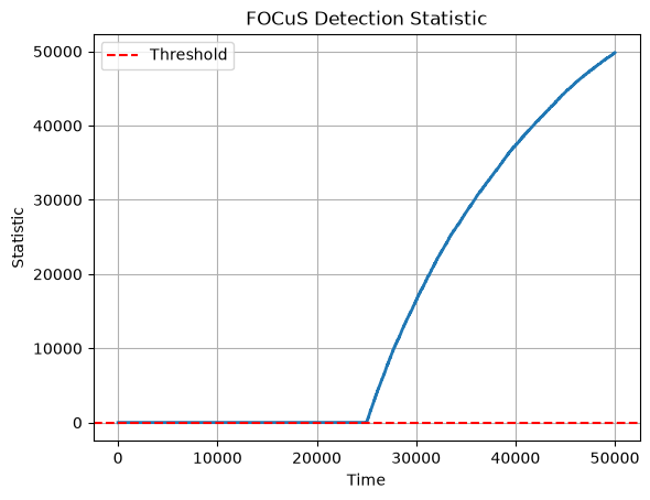
Passing threshold=np.inf computes the full trajectory of the test statistic without stopping, which is handy to study the behaviour of the statistic and pick a sensible threshold:

res_full = focus_offline(Y, threshold=np.inf, type="univariate", family="gaussian")

plt.plot(res_full["stat"], lw=2)
plt.axhline(25.0, color="red", linestyle="--", label="Threshold")
plt.xlabel("Time")
plt.ylabel("Statistic")
plt.title("FOCuS Detection Statistic")
plt.legend()
plt.grid(True)
plt.show()

Beyond the Gaussian Case

The focus-cpt package can also detect changes in one-parameter exponential family distributions, such as Poisson change-in-rate, useful for count data, Gamma change-in-scale (or rate), for positively defined data, and Bernoulli change-in-probability, for binary data. For instance, detecting a change in rate over count data is as simple as:

np.random.seed(101)
Y_counts = np.concatenate((np.random.poisson(lam=2.0, size=1000),
                           np.random.poisson(lam=6.0, size=1000)))

res = focus_offline(Y_counts, threshold=13.0, type="univariate", family="poisson")
print("Detection time:", int(res["detection_time"]))
print("Estimated changepoint:", int(res["detected_changepoint"]))

Detection time: 1003
Estimated changepoint: 1001

A neat design feature of the package is that the detector state is independent of the statistic computed on it. This means that the same detector can be queried under different distribution families, without re-running the analysis:

np.random.seed(2024)
Y_counts = np.concatenate((np.random.poisson(lam=10, size=500),
                           np.random.poisson(lam=15, size=500)))

detector = Detector(type="univariate")
for y in Y_counts:
    detector.update(y)

result_gaussian = detector.get_statistics(family="gaussian")
result_poisson = detector.get_statistics(family="poisson")

print(f"Gaussian statistic: {result_gaussian['stat']:.2f}, "
      f"changepoint: {result_gaussian['changepoint']:.0f}")
print(f"Poisson statistic:  {result_poisson['stat']:.2f}, "
      f"changepoint: {result_poisson['changepoint']:.0f}")

Gaussian statistic: 6922.16, changepoint: 500
Poisson statistic:  280.08, changepoint: 500

Other options include one-sided detection (type="univariate_one_sided", to only flag increases or decreases), a known pre-change parameter (via the theta0 argument, e.g. get_statistics(family="gaussian", theta0=0.0)), and detection of transient anomalies (via the anomaly_intensity argument). For more comprehensive examples and applications, refer to the documentation on the project’s GitHub repository https://github.com/gtromano/unified_focus.

More examples

Non-Parametric Changepoint Detection with Unknown Distribution

The focus-cpt package also offers non-parametric changepoint detection through the NP-FOCuS algorithm. This is beneficial when the underlying data distribution is unknown or the change nature is unpredictable beforehand.

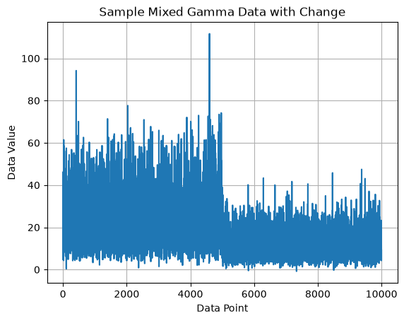
Here, we simulate data with a changepoint, but unlike previous examples, the data is a combination of Gamma distributions with added Gaussian noise, making the underlying distribution less clear.

np.random.seed(123)
# Define a simple Gaussian noise function
def generate_gaussian_noise(size):
    return np.random.normal(loc=0.0, scale=1.0, size=size)

# Generate mixed data with change in gamma component
gamma_1 = np.random.gamma(4.0, scale=6.0, size=5000)
gamma_2 = np.random.gamma(4.0, scale=3.0, size=5000)
gaussian_noise = generate_gaussian_noise(10000)
Y = np.concatenate((gamma_1 + gaussian_noise[:5000], gamma_2 + gaussian_noise[5000:]))

# Plot the data to visualize
plt.plot(Y)
plt.xlabel('Data Point')
plt.ylabel('Data Value')
plt.title('Sample Mixed Gamma Data with Change')
plt.grid(True)
plt.show()

With NP-FOCuS, we don’t make assumptions about the underlying data distribution. To achieve this, the algorithm monitors the empirical cumulative distribution function of the data at a set of quantiles. When you initialize the detector, you provide initial quantiles, such as the 25th percentile (dividing the data into fourths, marking the first quartile) or the median (splitting the data in half). These quantiles essentially act as markers to monitor different portions of the data distribution.

As new data arrives, NP-FOCuS calculates a separate statistic for each provided quantile, tracking how the distribution of data points around each quantile evolves over time. The detector then reports two aggregated statistics: the sum and the maximum across all quantiles. Monitoring the sum makes the detector sensitive to changes affecting the whole distribution, while the maximum is better suited to changes concentrated in one portion of it, e.g. in the tails. In our example, we monitor the 25th, 50th (median) and 75th percentiles, and place a threshold on the sum statistic:

# Initial quantiles estimated on training data (first 100 observations)
quantiles = [np.quantile(Y[:100], q) for q in [0.25, 0.5, 0.75]]

detector = Detector(type="npfocus", quantiles=quantiles)

for i, y in enumerate(Y, start=1):
    detector.update(y)
    stat_sum, stat_max = np.atleast_1d(detector.get_statistics(family="npfocus")["stat"])
    if stat_sum > 25:
        break

print(f"Change detected at time {i} (sum statistic: {stat_sum:.2f})")

Change detected at time 5019 (sum statistic: 25.99)

Multivariate Data

It is possible to run a multivariate analysis with a detector of type="multivariate", which implements the MD-FOCuS generalization, by feeding, at each iteration, a numpy array. Here’s an example of detecting a Gaussian change-in-mean over a 3-dimensional stream:

np.random.seed(123)

# Define means for pre-change and post-change periods (independent dimensions)
mean_pre = np.array([0.0, 0.0, 5.0])
mean_post = np.array([1.0, 1.0, 4.5])

# Generate pre-change and post-change data, with a changepoint at time 5000
Y_pre = np.random.normal(mean_pre, size=(5000, 3))
Y_post = np.random.normal(mean_post, size=(500, 3))
Y = np.concatenate((Y_pre, Y_post))

detector = Detector(type="multivariate")
threshold = 25.0

for y in Y:
    detector.update(y)   # feed one 3-dimensional observation per iteration
    result = detector.get_statistics(family="gaussian")
    if result["stat"] >= threshold:
        break

print(f"Change detected at time {result['stopping_time']:.0f}, "
      f"changepoint estimated at {result['changepoint']:.0f}")

Change detected at time 5014, changepoint estimated at 5000

For higher-dimensional streams (5 dimensions or more), the exact computation becomes expensive, and the package offers a fast approximation based on low-dimensional projections: see the generate_projection_indexes helper in the documentation.

Autocorrelated Data

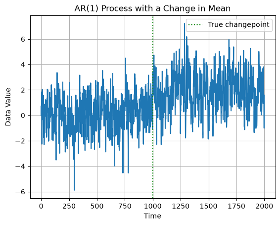
Real data streams often exhibit autocorrelation, which, if ignored, leads to frequent false alarms. The latest addition to the FOCuS family is a detector for a change in mean in the presence of autoregressive noise. We simulate an AR(1) process with a shift in mean:

np.random.seed(2024)

n, rho = 2000, 0.7
mu = np.where(np.arange(n) < 1000, 0.0, 2.0)  # mean shift at time 1000

# Generate AR(1) noise and add it to the signal
noise = np.zeros(n)
innovations = np.random.normal(size=n)
for t in range(1, n):
    noise[t] = rho * noise[t - 1] + innovations[t]
Y_ar = mu + noise

plt.plot(Y_ar)
plt.axvline(1000, color="green", linestyle=":", label="True changepoint")
plt.xlabel("Time")
plt.ylabel("Data Value")
plt.title("AR(1) Process with a Change in Mean")
plt.legend()
plt.grid(True)
plt.show()

The detector takes the autoregressive coefficients (rho, here treated as known — in practice, estimate them from historical data) and the pre-change mean (mu0_arp):

detector = Detector(type="arp", rho=[rho], mu0_arp=0.0)
threshold = 25.0

for y in Y_ar:
    detector.update(y)
    result = detector.get_statistics(family="arp")
    if result["stat"] >= threshold:
        break

print(f"Change detected at time {result['stopping_time']:.0f}, "
      f"changepoint estimated at {result['changepoint']:.0f}")

Change detected at time 1030, changepoint estimated at 999

Despite the strong autocorrelation, the change is detected quickly and located within one observation of the truth. For details on the underlying methodology, see our preprint on changepoint detection in the presence of autocorrelation.

Conclusions

In conclusion, focus-cpt is a versatile and efficient Python package for online changepoint detection. Whether you’re dealing with univariate or multivariate data, known or unknown distributions, independent or autocorrelated observations, focus-cpt has got you covered.

For a full comprehensive read on the methodology and both implementations, check out the software paper:

G Romano, K Ward, Y Fan, G Rigaill, V Runge, IA Eckley, P Fearnhead (2026). focus and focus-cpt: Fast Online Changepoint Detection in R and Python. arXiv preprint arXiv:2607.19961.

And again, if you prefer the R interface, the same functionalities are available in the focus R package: visit the introductory guide for R. For any question, don’t hesitate to drop me a message :)