Can Hamiltonian Win At Monte Carlo?
31st January 2016
As I said in my last post, Optimising with Ants and Ice-cream Cones, the MRes students at
STOR-i are currently in
a fornight of lectures giving brief outlines of research areas at Lancaster University. The rest of the week consisted of
three different topic.
On Tuesday, it was Dynamic Programming (DP) that was the main topic. Under this,
Chris Kirkbride gave us an introduction to DP
as well as talking about the problems of it when scaling. Then
Peter Jacko went further into this topic and introduced us to the idea of restless bandits. The session was concluded
by Professor Kevin Glazebrook with our first real
introduction to the Multi-Armed Bandit Problem. He also gave an explanation of the Gitten's Index that I spoke about in
Why Not Let Bandits in to Help in Clinical Trials?.
On Wednesday, the main topic was Computational Statistics, as was given by Chris
Sherlock and Peter Neal, both part of the Mathematics and Statistics
Department. Friday was on the use of Wavelets and Changepoints, given by Idris Eckley,
Matt Nunes and
Azadeh Khaleghi. These were both interesting topics, involving
some clever ideas.
The main thing I would like to talk about was a little comment made by Chris
Sherlock during his part of the Computational Statistics talk. He gave the basic idea of Hamiltonian Monte Carlo (HMC)
and how it can simulate from a difficult posterior distribution. A variant on HMC for Big Data was briefly mentioned in
Can MCMC Be Updated For The Age Of Big Data?, but I didn't go into the mechanics in much detail, focussing
mainly on its performance. I thought it was a wonderful idea, possibly because my background
is in physics and so using those principles appeals to me. I decided to look it up quickly and write about how it works. Unfortunately,
if you decide to search for "Hamiltonian Monte Carlo" online, you mainly get information about Formula One's Lewis Hamilton and the
famous racetrack in Monte Carlo. Eventually I found a paper by B. Shahbaba, S. Lan, W. O. Johnson and R. M. Neal, which begins by going
through the basic ideas.
Hamiltonian physics is based around a function called the Hamiltonian, $H(p,q)$. This quantifies the energy of a particle and is
a function of its position $q$ and momentum $p$. In many cases, the Hamiltonian is the sum of the particles kinetic energy,
$K(p)=p^TM^{-1}p/2$ (where M is a diagonal matrix representing mass),
and its potential energy, $U(q)$. If one considers the case of a particle near the earth's surface with on gravity acting upon it,
$U(q)$ is (approximately) proportional to the particles height above ground. From the Hamiltonian, one can calculate the trajectory
of the particle from the partial differential equations that each component of $q$ and $p$ satisfies Hamilton's equations:
$$\frac{dq_i}{dt} = \frac{\partial H}{\partial p_i} = \frac{\partial K}{\partial p_i},\qquad
\frac{dp_i}{dt} = \frac{\partial H}{\partial q_i} = \frac{\partial U}{\partial q_i}.$$
This has been very cleverly applied to Bayesian Statistics to simulate from non-standard distributions. Let $q$ be a vector of
parameters from the posterior distribution with prior $\pi$ and likelihood $L$. Then we can set
$$U(q) = - \log(\pi(q)L(q)).$$
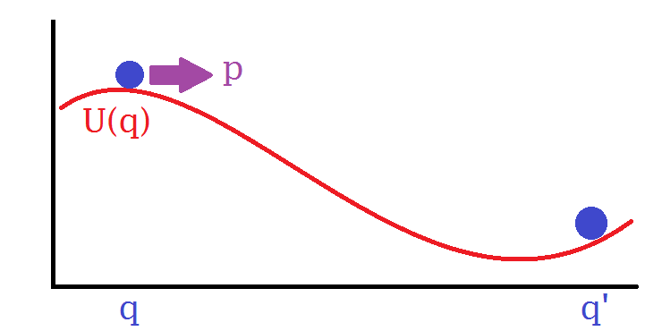
This inverts the posterior, and provides a potential (which can be considered a landscape) in which a particle can slide around.
Now that we have a Hamiltonian, each component of $p$ can be taken from a normal distribution with variance $M_i$, and the particle
at $q$ can be given this momentum. The particle will slide around the distribution, and exchanging kinetic and potential energy as it
traverses parts of the posterior with different heights. After a certain amount of time, the position
will be read again which, in principle, can be found from the Hamilton's equations.
The aim is to sample from the distribution. If your current sample is $q_i$, then a new sample point can be proposed by generating a
set of momenta in each dimension of the parameters, letting the particle slide around the potential for a given time, $t$, and then
choosing its position at time $t$, $q_{i+1}$. A Hamiltonian physics is invariant under certain transformations, the acceptance
probability is 1.
Unfortunately, it is often too difficult to solve Hamilton's equations exactly, and so numerical integration is required. This
leads to approximations creeping into the calculation and so the acceptance rate may not be exactly 1. Another problem is what
time step should we choose? Too short and we will hardly move anywhere and mixing of the posterior will be very slow. Too
long and the numerical integration will have too high a computational cost.
I really enjoyed looking into this, and thinking about it in a physical manner. My background in physics has got me thinking about whether
or not other ideas could be applied to these ideas. For example, could Langrangian mechanics (which involves the least action principle)
be used to solve similar problems. Or could you treat probability densties as forms and use the mathematical principles in general
relativity to move around them more efficiently. Unfortunately, I feel that the differential equations woul be even more computationally
difficult than the simple cases of Hamiltonian physics.
References
[1]
Split Hamiltonian Monte Carlo, B. Shahbaba, S. Lan, W. O. Johnson and R. M. Neal,
Statistics and Computing, Vol. 24(3), pp. 339-349 (2014)