Estimating Near Invisible Populations
3rd March 2016
We are very fortunate at STOR-i, as all sorts of opportunities come our way that we probably would never have had otherwise. We have
just had another Masterclass over two days given by Professor Ruth King
of School of Mathematics at the University of Edinburgh. Her Masterclass is entitled "Practical Bayesian Statistics" and is mainly
considering the practicalities of using Bayesian Statistics in a real study. The particular example she is discussing with us is how
to estimate the size of a population when it is either infeasible to count everyone or it is impossible. Examples of this include
the number of people who are injecting drugs, or the number of rough sleepers in a city. These sorts of counts can be hard as some
people hide the fact and how could you be sure that you had counted everyone?
To estimate the total number, one sends out multiple searchers and each searcher makes a note how many observations they make plus a
piece of information that uniquely identifies an observation. If the observations were people, it could be their name, for tigers it
could be the unique stripe pattern. It is important that the members of the population can be distinguished from one another, otherwise
the theory doesn’t work. For simplicity, consider the case when there are 3 sources of information. Let $i=1$ if an individual is seen
by source 1 and 0 otherwise, and similarly for $j$ regarding source 2 and $k$ regarding source 3. Then we let $n_{ijk}$ be the number
of individuals that satisfy the values of $i, j$ and $k$. For example, $n_{101}$ are the individuals seen by sources 1 and 3 but not 2.
By splitting the observations into these categories we find we have a partition of all the observations (no individual is in more than
one group). Therefore, to find the total number of individuals, $N$, we simply calculate
$$N=\sum_{i,j,k}n_{ijk}.$$

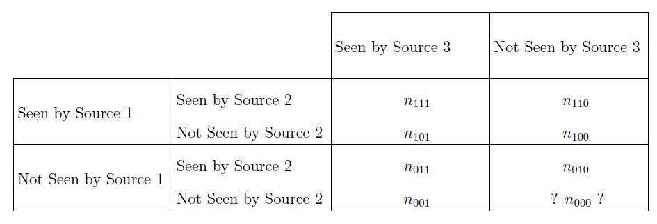
This table shows the different categories of which individuals were seen in which sources. The only unkown value is $n_{000}$ which is what we aim to estimate using Bayesian statistics.
The difficulty comes from the fact that $n_{000}$ is unknown. It is here where the statistics comes in. We assume that $n_{ijk}$
conditional on a rate parameter $\lambda_{ijk}$ comes from a Poisson distribution with mean $\lambda_{ijk}$. On top of this, we
assume that $\lambda_{ijk}$ has a log-linear regression model with parameters representing an underlying mean, $\theta^0$, main
effects from each source and interactions between sources. Each parameter is assumed independent. If we have beliefs about the
sorts of values these parameters should take, then we could add a prior $p(\boldsymbol{\theta})$ that is the product of the priors
for each parameter. After this, an MCMC algorithm can be used to sample from the posterior for $\boldsymbol{\theta}$, from which we
can estimate $n_{000}$. So far, this is fairly standard stuff, just "turning the Bayesian crank" with nothing really new.
One of the problems Prof. King spoke about was how to incorporate the information given to you by an “expert” into the prior beliefs.
For example, the interactions between sources could be either positive or negative. An expert may be fully convinced that it should
be positive, but putting this directly into the model by, for example, using a normal distribution restricted to the positive axis
$N^+(0,\sigma^2)$, would mean that no matter what data said to contradict this belief, it could never override the experts’ opinion.
Even experts can be wrong though, so Prof. King suggested that a more sensible method would be to use a weighted sum of positive and
a negative normal
$$(1-\omega) N^-(0,\sigma^2) + \omega N^+(0,\sigma^2)$$
where $\omega$ is a high probability (eg. 0.95).
The final message Prof. King left us with was to make sure we really understood the data that we are dealing with. Her example was when looking at current injecting drug users. There were four different sources, one of which came from a Hepatitis C register. When using this data, the data showed a big increase over time of injecting drug users, completely contradicting what the experts thought. Granted, experts can be wrong, but it brought into question whether the model was correct. Further investigation showed that the Hepatitis C register included both past and current drug users and so gave an overestimation of the true value of $n_{000}$. Once this had been spotted, the model could be adjusted to account for this. However, this slight misunderstanding of what the data could have led to very big errors. Thus, it is very important to really engage with experts so that one knows as much as possible about the data and how it is collected.