Von-Neumann, risk, and birds: How to model rational behaviour

The idea of expected utility is one that attempts to mathematically model the choices individuals make under uncertainty. These are often complex situations, with a key parameter being the risk appetite for the situation. Here, the term “risk appetite” pertains to the level of risk one is willing to take in order to obtain an objective and these could range from something as fundamental as getting enough food for survival, to trying to win big in the lottery. Expected utility settles itself within a wider cacophony of approaches towards decision-making under risk, and is arguably the most prominent and followed noise.

As early motivation, consider a decision maker who is faced with with a set of outcomes, each with their own associated risk. Under expected utility, the main assumption is that the decision maker will aim to maximise the expected value over all possible outcomes. The function that contains all possible outcomes is referred to as a utility function and is the fundamental concept when trying to explore expected utility, especially from a mathematical perspective.

This blog aims to follow rational decision making from a mathematical viewpoint, starting from its formalised origins in the 20th century, although the ideas date back to the 18th century. With this, the four essential components to what makes a decision maker rational is presented; this is then followed by a primer on utility functions based on a school of thought known as Von Neumann-Morgernstern theory. To bring home understanding, we fly through an example that applies the theory to a problem involving the utility of food. Following this is an extension and consideration of shifting rational behaviours and a wrap up with some further theory and practical applications.

Rationality through a mathematical scope

In its mathematical sphere of interpretation, the theory stemmed from work by prominent economist Oskar Morgenstern (also attached to this project was some little known footnote mathematician, John Von Neumann). Explored in the opening of Section 3.2 in Ken Binmore’s fantastic book, “Rational Decisions“, it was said Morgenstern had approached von Neumann to help formalise ideas in another field known as Game Theory. Together they developed and released the “Theory of Games and Economic Behaviour” in 1944 which packaged and cemented some neat initial results in game theory.

As a precursor to all the mathematics presented, Morgenstern was irrationally persistent in wanting the exhilaratingly high octane issue of cardinal utilities, which had been used fruitfully throughout the book, well defined and given as a basis for which their game theory ideas built upon. So as one does, Von Neumann invented a theory on the spot which measures a person’s preference to something based on the risk they are willing to take to attain it. Thus, we arrive at von Neumann-Morgenstern Theory (or VNM Theory from here forth).

Their ideas can be cemented through a set of four postulates. Under a mathematical context, postulates can be thought of as statements that are accepted as definitively true without having necessarily to prove it as such. Von Neumann and Morgenstern didn’t particularly provide the most approachable explanation of these postulates, however they can be summarised in laymen’s terms as follows.

These four postulates when satisfied constitute what is believed to be a rational decision maker. And from this, their preferences can be modelled by what is known as a utility function. But what is this?

Navigating the rabbit hole of utility functions

A key subset of the theory, utility functions, models a preference relation between utility and some
measurable quantity (wealth, food, etc.), the incorrect assumption of a utility function is something that
often occurs and leads many to come up with incorrect, and sometimes nonsensical musings on rational behaviour. A good example not explored here is the St. Petersburg Paradox, which can help the reader understand what occurs when incorrect rational behaviour is assumed. Utility functions are essentially ways in which we can express preference as a set of ordered rankings in which we assign a utility metric known as utils to each. With this, we aim to find the expected value and to subsequently assess and explain risk preferences for individuals.

Utility functions are required to have satisfied the four axioms from VNM Theory, and can be
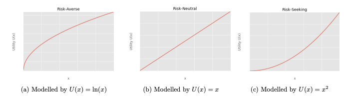
utilised to measure and model risk appetite. Under VNM theory, these attitudes to risk are consistent throughout, with three categories being risk-averse, risk-neutral, and risk-seeking behaviours. The first
of these is represented by a function that will slow down over time (formally defined as a concave function) and provides a preference for low variance outcomes. A risk-neutral individual is indifferent towards an outcome and can be represented by a function of just a straight line (affine). Finally, risk-seeking individuals will have more utility in achieving a higher level of outcome, therefore their function increases quicker and quicker over time (convex function). These functions are expressed in terms of U(x), which maps some quantity x such as food or wealth, to utils, an aforementioned unit for utility.

A very important addendum to all this is that these functions, and the values they produce, cannot be compared like regular numbers. Utility under this setting requires that if one value of utility is higher than another, it is just objectively preferred and not preferred so many times more than another. Take for example: if for events x_1 and x_2, U(x_1) = 42 and U(x_2) = 3, x_1 is not 14 times more preferred than x_2.

The Birds!

We can consider a quick example to see how different risk appetites arise, and how both a fixed utility function, or a variable utility function can be applied to the situation. To do this we can consider the choice a bird makes in the face of hunger.

To get rid of the trivial idea you may have that it’s not particularly feasible for a bird to be making rational human decisions. Consider some kafkaesque-light bird with some human psyche engrained within its internal cognitive function. I.e. This is not your senseless bird running amok in Bodego Bay; this is a rational bird, making rational decisions.

Now, this bird is fairly hungry, and needs some food to scavenge for, say x amount over an arbitrary amount of time. The bird has the choice as to whether go beyond what they usually are able to gather and risk dying in the process (obviously returning with nothing as they’re dead) or settle for an amount they know is safe and can be collected rather quickly.

The rational choices this bird can make, and the utility it attains from such, can be partitioned into a few scenarios:

• Scenario 1: (the bird is starving): In this scenario, a risk-seeking approach would need to be made to attain enough food for survival. To make sure this is reflected in their utility function, it would be required to see the bird value the expected utility from the amount of food it finds over the average amount of food it’s expected to find, and thus forage for food even if it’s more than should be expected.

• Scenario 2: (The bird likely has the means to attain ample amounts of food under both scenarios):
  Here, they are indifferent to the amount of food they’re expected to get, and the utility it attains from this. Therefore, it does not value taking the risk and potentially gaining a greater payoff, than it does going for a safe amount.

• Scenario 3: (The bird likely only needs a small amount of extra food): Finally, here the bird only requires a small amount of extra food and is willing to take a safe payoff for this, even if it’s less than the amount they usually expect to get.

Now, the first time I grappled with the avian madness and the overarching concepts as a whole, i found myself descending into a tangle to fully understand how this represents our decision making under risky situations. With scenes at the time of my brain trying to explain this to me roughly amounting to this:

Therefore, I often found it best to run through some numbers and to check the scenarios descriptions against the graphs of the different utility functions we saw earlier. So let us do just that:

Evaluating Scenario 3:
Here, the bird has enough food to survive, thus it is said to be risk-averse as explained in the scenario setting. From this, it’s utility function for the food quantity x could be something like ln(x) (the natural log), which is just the example function given in the earlier graphs of the previous section. From the worded description of the scenario, if we was to think of this in terms of expected value of the amount of food we expect to attain, what we are saying is that the utility of the expected value should be worth more than the expected utility. Specifically the amount of food we are expected to attain is a safe bet for us to take.

You can see how this is reflected in the chosen utility function for risk-averse behaviour by plugging in some values. Say for example we have an equal chance of attaining 2 amount or 7 amounts of food (whether that be kg, grams or some other metric is irrelevant here). Then the utility for the expected amount is just the mean of these numbers plugged into the utility function, or,

U\left(\frac{7+2}{2}\right)=U(9/2)=\ln\left(\frac{9}{2}\right).

The expected value of the utility is analogously calculated as:

\mathbb{E}\left[U(7)+U(2)\right]=\frac{\ln(7)+\ln(2)}{2}=\frac{\ln(14)}{2}

Using a calculator, it should be found that \ln(9/2)\geq \ln(14)/2, so taking the safe option of the expected amount has more utility to us in a risk-averse scenario, this is what was described earlier. Checks can also be done for the first two scenarios, but here we expect to value the expected value of the utility more and equally respectively.

Conclusion

This is all well and good modelling the Bird having a strict concept of rational behaviour and having a consistent approach to the matter. But what if the situation changes and evolves as we attain more food? What if the bird no longer the feels to value food as much as it once did? Or what if disaster strikes and food suddenly becomes a luxurious scarcity. The suspense is palpable!

We can answer such intriguing questions in a future blog post!