This post is all about the game of blackjack. What is the optimal strategy? How much money can you expect to win on average, if you play optimally? Should you decide to play at all?
The first section will outline the formulation of the rules we’ll be considering. We’ll then mathematically define the task at hand by formulating the problem as a Markov decision process, and solve it with linear programming.
Blackjack
Blackjack is a card game where the aim is to collect cards totalling a value higher than that of the dealer without exceeding 21. The game begins with the dealer dealing a card to each player and themself. The cards have the following values: 2-10 are worth their face values, picture cards (jack, queen, king) are worth 10, and aces can be counted as either 1 or 11 according to choice. On their turn, players have two choices: hit (be dealt another card from the deck) or stick (stop drawing cards). If the total value of a player’s cards exceeds 21 they go bust and immediately lose, receiving a reward of -1. After all players have opted to stick, it is the dealer’s turn. The dealer plays according to a fixed strategy where they hit on any total up to 16 and stick on 17 or above. All remaining players win (receiving a reward of 1) if the dealer goes bust. Otherwise, remaining hands win if their total value is higher than the dealers, draw (receiving a reward of 0) if it is the same, or lose if it is lower.
We’ll assume that the cards are dealt from a deck that is sufficiently large that the probabilities of drawing any particular card do not change significantly over the course of the game, so that draws from the deck can be modelled as independent and identically distributed and there is no benefit to keeping track of the history of cards dealt to yourself or other players. This is not an unrealistic assumption for casino play, where cards are dealt from a shoe of several decks that is periodically re-shuffled, and card-counting is frowned upon anyway!
This means that each player can be considered to play independently against the dealer. It also means that only three pieces of information are required to decide which action to take next: the player’s current total (with an ace counted as 11 unless doing so results in a total over 21), the dealer’s card, and whether or not the player has an ace that is currently being counted as an 11. The last situation is known as having a usable ace or a soft hand, since the player can save themself from going bust by instead counting their ace as a 1.
Formulation as a Markov decision process
A Markov decision process (MDP) is a sequential decision-making process where outcomes depend on the decision maker and are partly random. At each time step, the player finds themself in some state S \in \mathcal{S} and must select some action A from an action set \mathcal{A}(S). After taking an action, the process moves to the next time step, moving randomly to some new state S' (the probabilty of moving to any particular new state will likely depend on the action taken) and awarding a reward R(S,S') to the player.
In blackjack, the possible states are triples of three numbers (s,d,a) , where s \in \{2,\ldots,21\} is the player’s current total, d \in \{A,2,\ldots,10\} the dealer’s card, and a \in \{0,1\} is whether the player has a usable ace (a=1) or not (a=0). In each of these states, the player has two possible actions: hit or stick. We also have three special terminal states: WIN, DRAW, and LOSE. When a player reaches one of these states they are awarded with the rewards 1, 0, or -1 respectively and can no longer take any actions or receive further rewards.
The possible state transitions are as follows:
If the player sticks on some total s, they transition to WIN with probability \mathbb{P}(\text{dealer goes bust or sticks on total less than s}), DRAW with probability \mathbb{P}(\text{dealer sticks on total of s}), or LOSE with probability \mathbb{P}( \text{dealer sticks on total greater than s}). These probabilities can be computed exactly by recursion (this is a little fiddly since there’s lots of cases to consider, but is possible since you can’t visit the same state twice), or estimated by simulating a large number of hands for the dealer and observing how often they stick on 17, 18, 19, 20, or 21 and how often they go bust (much easier!). The exact probabilities are represented in the figure below:
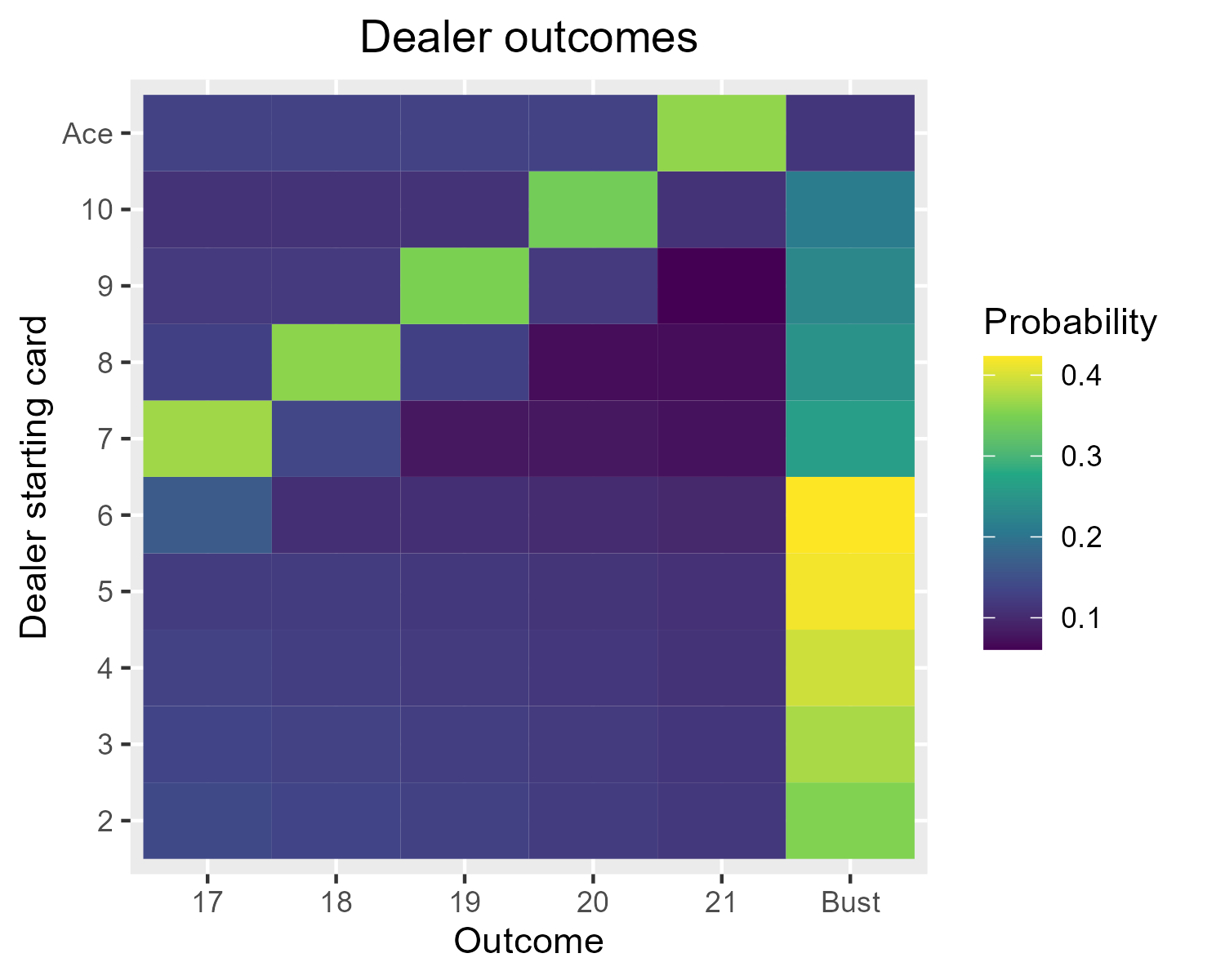
Note that these are mostly dominated by the fact that drawing a 10 occurs with probability 4/13, so starting from a 7 the most likely outcome is to end up sticking on 17, but starting from a 6 the most likely outcome is to go bust after hitting on 16.
If the player hits, the transitions are a little more complicated. First a card of value c is drawn from the deck:
- If s \leq 10, the player cannot go bust and we transition to state (s+c, d, a) (if an ace is drawn, we count it as an 11 so c=11 and a = 1).
- If s \geq 11 then we always count new aces as 1 (since counting it as an 11 would cause us to go bust). It is now possible for the player to go bust:
- If c \leq 21 - s, we transition to state (s+c, d, a).
- If c > 21 - s and a=1, we must use the ace and transition to (s+c-10,d,0) .
- If c > 21 - s and a=0, go bust: transition to LOSE and receive reward -1.
Optimal strategy
Our objective is to find the decision strategy that maximises the expected reward. This can be represented as a function \pi^*(S) of the current state that tells us the best decision to take. To find this, it will be useful to define one last concept: the value v(S) of being in a particular state, i.e. the expected reward if we start in that state and play optimally. For a MDP, these values exist and are uniquely defined as satisfying the Bellman optimality equations:
\begin{aligned}v(S) &= \mathbb{E}(R(S,S') + v(S') \, | \, S, A = \pi^*(S)) \, .\end{aligned}
That is to say, the value of being in state S is the expected value of the immediate reward received plus the value of the state we transition to, given that we start in state S and take the optimal action \pi^*(S).
In particular, since \pi^*(S) chooses the action that maximises expected reward, this means that:
\begin{aligned}v(S) &= \max_{A \in \mathcal{A}(S)}\mathbb{E}(R(S,S') + v(S') \, | \, S, A)\\ &= \max_{A \in \mathcal{A}(S)} \sum\limits_{S' \in \mathcal{S}} \mathbb{P}(S' \, | \, S,A) (R(S,S') + v(S')) \, . \end{aligned}
The v(S) therefore satisfy the following inequalities:
\begin{aligned}v(S) \, &\geq \, \sum\limits_{S' \in \mathcal{S}} \mathbb{P}(S' \, | \, S,A) (R(S,S') + v(S')) \quad \quad \forall A \in \mathcal{A}(S) \, ,\end{aligned}
with equality for A = \pi^*(S) .
This means we can find all of the state values by solving the following linear program:
\begin{aligned}&\min\limits_{v \in \mathbb{R}^{|\mathcal{S}|}} \; \sum\limits_{S \in \mathcal{S}} \,v(S), \\ \\ &\text{subject to:} \\ & v(S) \, \geq \, \sum\limits_{S' \in \mathcal{S}} \mathbb{P}(S' \, | \, S,A) (R(S,S') + v(S')) \quad \quad \forall A \in \mathcal{A}(S) , \; S \in \mathcal{S}\end{aligned}
The minimisation objective and \geq constraints mean that the solution to the problem will be the unique set of values that satisfy the Bellman equations. The linear program can be efficiently solved with eg. the simplex algorithm as long as the state and action spaces aren’t too large, which is the case for our formulation of blackjack.
We will then be able to recover the optimal strategy \pi^* as:
\begin{aligned}\pi^*(S) &= \argmax_{A \in \mathcal{A}(S)} \mathbb{E}(R(S,S') + v(S') \, | \, S, A) \, .\end{aligned}
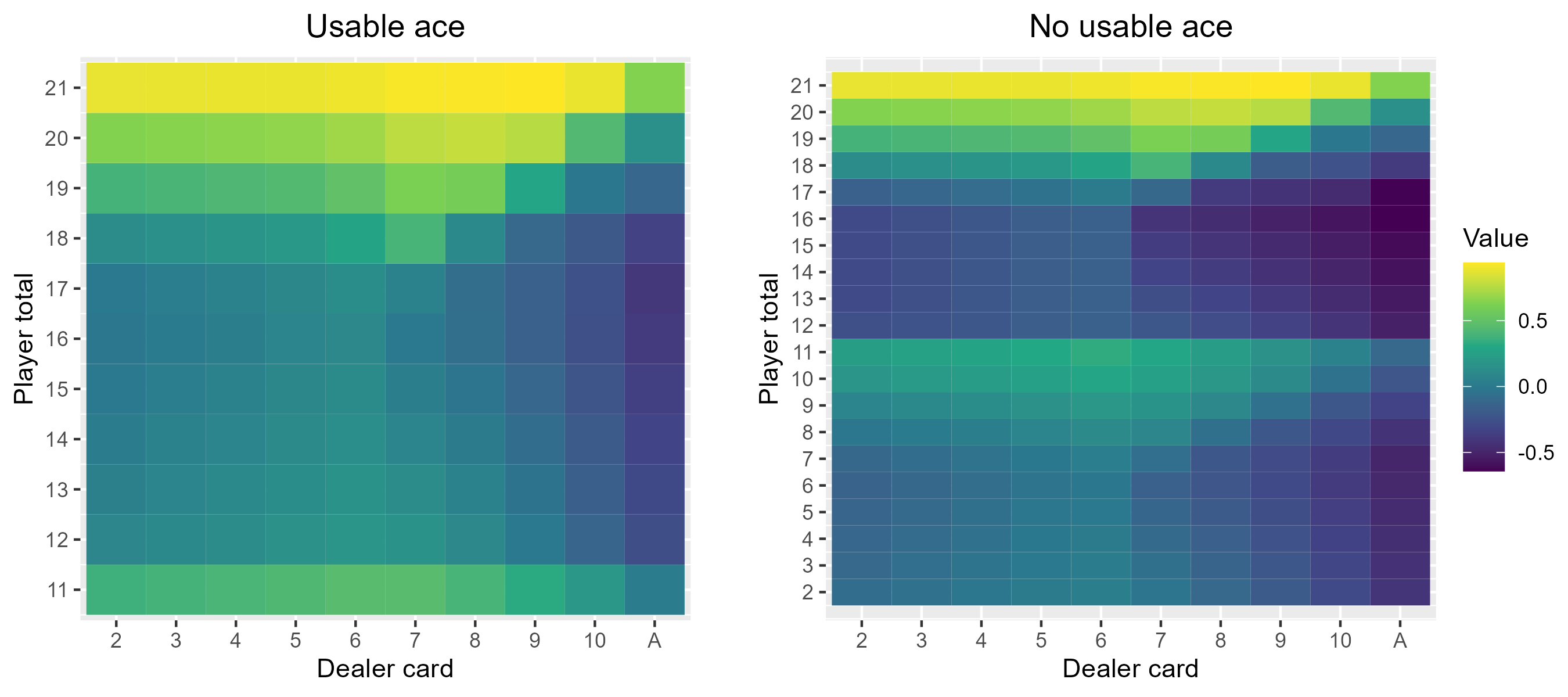
What does all of this look like for blackjack? Using the above method, the values of all of the possible blackjack states are as follows:
And, to answer one of the questions I asked to start with, the optimal blackjack strategy is:
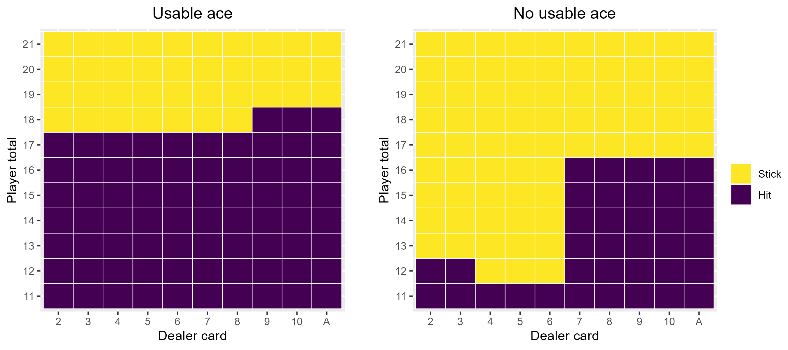
Note that you should obviously also always hit on totals up to 11.
Time to play blackjack?
Not quite. The other question of relevance is how much money you can expect to win! Since we know the probabilities of all of the possible starting states, as well as the values of starting in all of them, we can also compute the expected value of the game. That value is… -0.0466. Unfortunately, even playing optimally we can expect to lose money. This is largely due to the fact that if the player goes bust they lose immediately – we don’t check to see if the dealer would have gone bust as well so there is no chance of a draw (if we did then we would expect to win a princely 0.136). The same holds true when the player has the option of splitting or doubling, although the house edge is smaller. This is by design – if there were no house edge then blackjack would not be a casino staple.
So unfortunately, the real winning move is not to play at all. Alternatively, if you’re playing with friends, make sure you volunteer to be the dealer!
Further reading
- Optimal Blackjack Strategy Using MDP Solvers – Kunal Menda
- Reinforcement Learning : An Introduction – Sutton, R. S. and Barto, A. G.