I thought I’d write here about one of the things in my job that lead me to start thinking about statistics again and therefore to STOR-i. As a credit risk analyst, a large part of my job involved monitoring and adapting models for clients which incorporated scorecard models into them. I never actually got to build a real model myself but as a fun training exercise we had a model building competition
What is a credit scorecard?
Within industry, credit scorecards are used to assign a score to an individual which gives you a gauge on their predicted riskiness. This riskiness is based on predicting the probability of default which can vary in definition but in general will be a chosen set of criteria which indicate a customer is unlikely to pay. They are very useful as it’s simple to explain how to use them to a non-technical audience which is often key when boards of directors need to understand why decisions have been made or perhaps individuals wonder why their application for a loan has been declined.
A scorecard may generally look like the following:
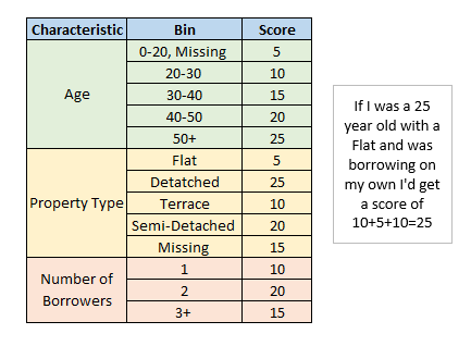
To use this scorecard you’d go through each characteristic and assign the correct score for that individual, adding these up to get a total score. Just to note the scorecard above is extremely simple and was created on the fly by me so don’t take this to have any actual predictive power. A properly built scorecard would contain many more variables and may use some scaling which takes the raw score and transforms it to get a final score. A common scaling would be multiplying by 20/log(2) and adding 500 as this multiplier leads to a final score where an additional 20 points onto the score doubles the odds (this is the probability being predicted divided by 1 minus the probability).
Types of credit scorecards
There are two types of credit scorecards:
- Application scorecards. These predict the probability an applicant will behave in a certain way based on data you would gather on application (for a loan for example). They are used in the decision process for acceptance or rejection for approval of the application but also may be used during the lifetime of the loan to judge if there has been a significant increase in risk since the application.
- Behavioural scorecards. These are scorecards that are based on data gathered through the lifetime of the loan or mortgage. This can be things such as paying habits or changes in circumstances. In particular, I saw these used to predict the probability of default and the probability of redemption which were used as part of a calculation of expected losses (IFRS9 and IRB).
How can you build a credit scorecard model?
There are different methods that can be used to build a scorecard but I’ll talk you through the method I’m most familiar with:
Step one: Gather and clean your data.
If you are working with real life data, you can have erroneous data which you want to get rid of or change prior to trying to build a model with it. For example, if you have a case where there was a default date set whenever the data was missing, then you would have to appropriately deal with this if that date was going to be used in variable in the model (perhaps a “time since X happened” variable). Your data pull needs to include data from an observation point in time (this is the data you will build the model on) and data to determine an outcome (for probability of default models this is whether a default occurred within the outcome period or not).
Step two: Create any new variables
You might want to create some new variables which combine two characteristics or represent a history rather than just having point in time data. Here this would include deriving the an outcome to each observation (if this wasn’t easily found in the first step).
These outcomes are often referred to as:
- Goods – if the event you are predicting didn’t occur.
- Bads – if the event did occur (e.g a default).
- Indeterminates – if you couldn’t determine whether the event occurred or not.
Step three: Split the data
Randomly split the data so you have a development sample to build the model with and a testing sample which you can use to test the model once it is built. A common split is 80% development and 20% testing.
Step four: Fine classing
Put your possible model variables into an initial set of bins. You want to keep this quite granular at this stage so you might have a large number of bins (perhaps up to 20). For example you could split a variable like property age into 5 yearly splits, so you’d have 0-5, 5-10 and so on with a bin at the end for anything exceeding your final bin value and another extra bin for missing values.
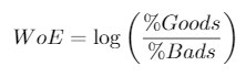
Step five: Calculate WoE and IV
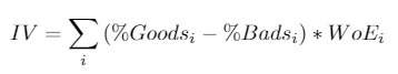
For each bin of each characteristics you need to calculated a metric known as the Weight of Evidence (WoE). This is the natural log of the percentage of goods that fall into this bin for this characteristic from your sample divided by the percentage of bads that fall into this bin for this characteristic from your sample. This will be used in the next step but is also used to calculated the information value for each characteristic. This takes the difference in the percentage of goods and bads multiplied by the weight of evidence, summed up for each bin. Here are the formulas
Step six: Coarse classing
Based on similar WoE evidence values we can group together bins to create larger and less granular groups for each characteristic. At this stage we can also remove some variables from consideration based on their IV as a low information value will indicate low predictive power. It is good to keep recalculating the WoE and IV as you group bins together to keep checking you are making the right decisions.
Step seven: Choosing a dummy variable or WoE approach
Both approaches will yield similar results but in certain situations one will perform better than the other. For example the weight of evidence approach is good when you have a lot of categorical variables but the dummy variable approach is simpler.
Dummy
This involves splitting your coarse classed variables up so each bin has its own binary dummy variable which will take the value of 1 if an individual falls into that bin for the characteristics or 0 if not. In this case there will be a different coefficient assigned to each dummy variable.
Weight of Evidence
Keeps each characteristic as a single variable but for an individual the variable takes the WOE value corresponding to the bin they fall into. In this case there will be a single coefficient assigned to each variable
Step eight: Logistic regression
Now it’s time to build the model (Yey!). You can do this using programs such as SAS, R and Python. Logistic regression is used to model probabilities of events which have 2 possible outcomes and gives you a predictive model which looks like the following:
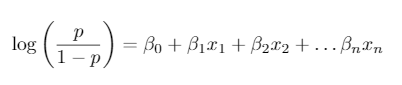
Here the left hand side of the equation is the log odds where p is the probability you are trying to predict.
Step nine: Check model against test data
Once you’ve built your model you can apply it to the test sample you kept aside in step three and see how well it is performing.
Step ten: Change it a scorecard format
If you decided to use a dummy variable approach then the score assigned to each bin for each characteristic is just the coefficient of the corresponding dummy variable. If you went with the WoE approach you will need to multiply the coefficient for that characteristics variable with the WoE for the bin you want the score of.
Scorecard monitoring
There are a number of standard metrics used to monitor the performance of a scorecard. A main one is (as one might expect) comparison of the actual rates versus the predicted rates, this monitors that the model is accurately predicting what it should be however in the case it is not a basic calibration can be performed to bring these more in line. This just involves a gradient and intercept shift to the distribution of scores however more complex methods can be used. Another largely used metric is the Gini coefficient to measures the discriminatory power of the model. This looks at the distribution of goods vs bads and will higher if more of the goods have higher scores and more of the bads have lower scores (so a Gini coefficient of 100% would be perfect discrimination – though not necessarily a perfect model).