This post is part of series about IMRT Planning, if you haven’t read the introduction to this series you can find it here. This blog series was inspired by the research I did as part of STOR601.
What is the problem?
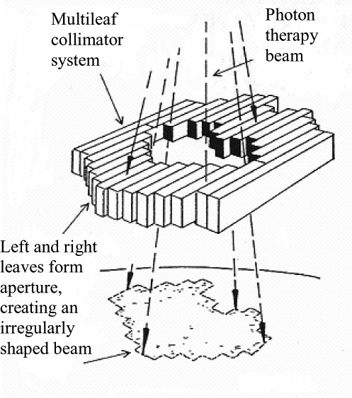
In IMRT the radiation delivered by the accelerator is one beam, but thanks to the multi-leaf collimator this beam can be imagined as a grid of “beamlets” or “bixels” that can be independently turned on or off. We can also (rather morbidly) imagine slicing the volume of tissue around a tumour into many cubes called “voxels”.
Given a small enough cube size then the tumour can be roughly modelled as a subset of all the voxels. Likewise, healthy tissue which we do not wish to irradiate can be modelled as a separate subset of voxels. The aim is to deliver a high amount of radiation to the tumour, but a low amount to the healthy tissue.
Given an angle, each individual bixel has a certain effect on each individual voxel. So for every angle (the angles given in BAO), the total intensity or strength of each bixel needs to be decided so that every voxel gets the correct total dose. Dosages are decided by the clinician.
More precisely, if x_i represents the decision variable for intensity of bixel i, b_i represent the required dose in voxel j, and A is the matrix such that a_{ij} is the dose delivered to voxel j per unit of x_i, then a simplified problem can be formulated as
A{\bf x} ={\bf b}
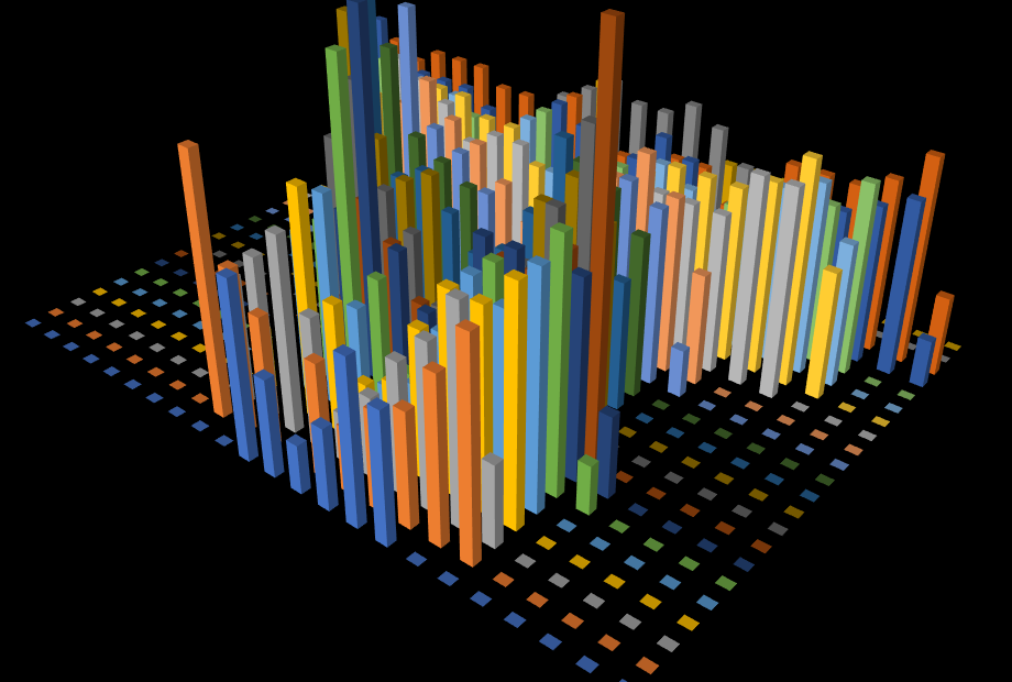
The {\bf x} vector determined here can be converted into a matrix to correspond with the grid of bixels. This is also know as a fluence map and hence the name Fluence Map Optimization or FMO.
What are the challenges?
The first challenge with solving this problem is that not every voxel contains only one tissue type. Since the voxels are a discrete approximation to continuous shapes that all share a boundary, then some voxels will contain a bit of cancerous tissue and a bit of healthy tissue.
This is problematic as it causes conflicting treatment goals. Do we provide a high dose to kill the cancer, but also kill the healthy cells? or do we provide a low dose to spare the healthy cells, but risk not getting rid of the cancer?
This is a tricky question as the tumour may be close to an important part of the body (such as the spinal cord) which if damaged could cause life-changing (or life-threatening) injury, although normally the cancer is the priority. Any formulation of the Fluence Map Optimization problem needs to take this into account.
Usually this manifests as what are known as dose-volume constraints. These constraints say that we must relax the conflicting constraints, but for only so much of the “at risk” tissue (healthy tissue we do not want to damage). The optimisation works out exactly what voxels go into that percentage to minimise risk of injury to the patient.
The second challenge is the scale of the problem. There can be a grid containing 100 bixels that the collimator can generate and 1000s of voxels to consider, and if dose-volume constraints are used then 1000s of binary variables for each voxel.
This makes the problem a lot harder to solve although popular ways of dealing with this challenge is by using techniques such as column generation and valid inequalities. One of my favourite formulations of this problem uses a concept from economics called conditional value at risk to produce dose-volume constraints that are linear (which makes solving this problem a lot easier).
What is the next step?
The next step in this process is to figure out the best way of delivering the dosage specified by the Fluence Maps for each angle.
Read about the challenges of Leaf Sequencing Optimization (LSO) here – Coming Soon!
Further Reading
Linear Programming approach to the FMO problem (One of my favourite approaches)