This post is part of series about IMRT Planning, if you haven’t read the introduction to this series you can find it here. This blog series was inspired by the research I did as part of STOR601.
What is the problem?
In the previous phase, matrices known as fluence maps were derived for each angle that will be used in the treatment plan. Most of the planning is complete at this stage. The planning process now focuses on working out the best way of bringing this plan into the real world using real equipment.
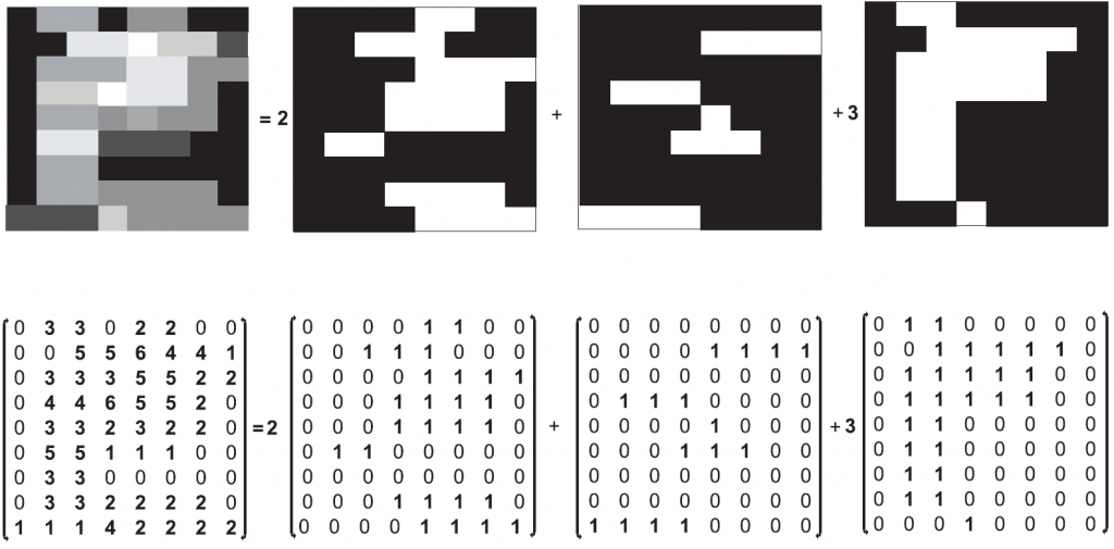
As mentioned in the introduction to this blog series, a multi-leaf collimator (MLC) is used to modulate the beam from the accelerator. The beam can be thought of as a grid of beamlets and a leaf can force a beamlet to be either on or off. Therefore, the problem is to decompose the fluence maps into a collection of 0-1 matrices (also known as apertures) that the collimator can deliver. This is known as Leaf Sequencing Optimization or LSO.
There are three main goals when solving this problem:
- Make the treatment deliverable: The angles and fluence maps from BAO and FMO respectively are the “blueprints” of the treatment, the LSO provides the “instructions” on how to build the treatment.
- Minimise the beam-on time: Beam-on time is the total length of time the accelerator is turned on for and needs to be minimised to increase patient comfort and quality of treatment.
- Minimise number of apertures: Minimising the number of apertures means that there is less time wasted changing between them.
What are the challenges?
The main challenge with this problem involves the physical limitations of different collimator systems. Gören et al. (2015) gives a really good review of using different collimator systems and they are summed up here:
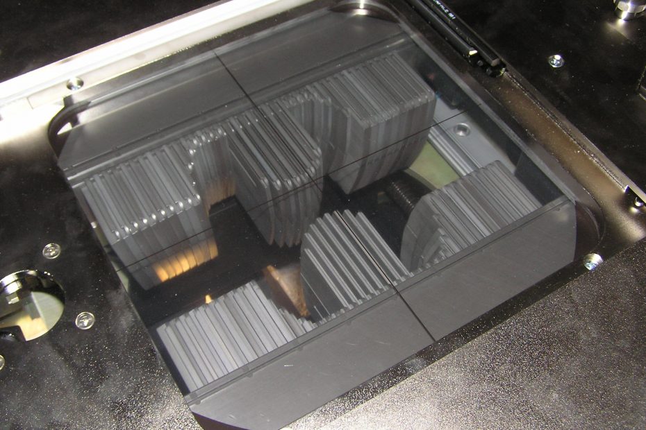
Regular MLC: As seen in the featured image for this blog post. Two sets of leaves, one left set and one right set, that can move in and out of the way of the beam. Notice that if the left leaf is covering a beamlet, then all beamlets to the left of that one must also be covered. This is similar in reverse for right leaves. This collimator also demonstrates what is known as the “consecutive ones” property where there has to be a continuous gap between ends of the leaves (no “floating” bits).
Rotating MLC: Similar to the regular MLC in every way except the whole unit can rotate 90 degrees to turn the left-right leaves into top-bottom leaves.
Dual MLC: Similar to the regular MLC except has a pair of left-right leaves and a pair of top-bottom leaves. This allows for more complex shapes to be made but is also harder to operate due to the potential collisions of the leaves.
Freeform MLC: This MLC is a purely theoretical collimator that can independently turn a beamlet on or off. This is useful to think about as it provides a starting decomposition that can be modified to work on a different collimator. If your algorithm or optimisation fails to find a decomposition for this MLC in good time (or at fails to find one at all!) then it’s a sign that your algorithm or optimisation will also struggle finding a decomposition for the others.
As can be seen from above, the number of constraints in your LSO problem depend heavily on the choice of collimator. There exist further constraints in some cases such as disallowing opposing leaves in adjacent rows to brush against each other (known as interdigitation), as well as potentially including maximum and minimum sized opening constraints.
The secondary challenge with the LSO problem is it’s complexity. The problem of minimising the sum of the total beam-on time and the total time taken to change between shapes is proven to be NP-Hard. Normally the time taken to switch between shapes is considered negligible and ignored.
This becomes an issue when trying to solve a perfectly fine mathematical model of the problem on a computer. A formulation can be fine on paper but can’t be solved quickly even using up-to-date commercial solvers on moderately powerful computers.
Therefore, research has been done in relaxing constraints in the problem and trying to exploit the structure of the LSO problem to use other mathematical optimisation tools, restating parts of the problem as network flow problems.
What is the next step?
In the traditional three phase approach, this was the final step! The planning stage is complete. Although the research doesn’t stop here. Improvements have been made to all phases individually, but there is promise in combining some of these steps in the hope that this increases the treatment quality and decreases planning/treatment time.
Further Reading
Formulation for LSO that looks good mathematical but is hard to implement
Column generation approach to the LSO problem
Decomposition of LSO into a collection of network flow problems