In this second and final blog in the series dedicated to analysing daily attendances in accident and emergency departments, we will attempt to forecast the daily number of attendances at A&E using three different forecasting methods. The first blog focused on exploring the data and identifying relationships between attendances/admissions and patients’ age/referral source/arrival date/time. To read the first blog (click here).
2.5 Decomposing the Data
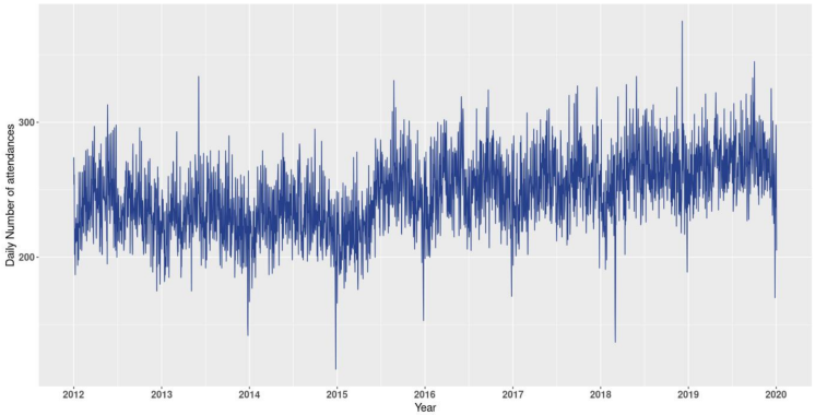
In 2015 the hospital of interest saw one of its neighbouring hospital’s ED close, as a result the number of attendances at the A&E suddenly increased. As seen in figure 9, the average number of attendances before and after 2015 are different. This could be accounted for using change point detection prior to implementing our forecasting algorithms. However, due to the nature of the change and also to simplify the problem and accurately forecast the time series, only attendances recorded between 2016 and 2020 were kept. (To learn more and read a blog on change point detection (click here)).
Figure 9: Daily number of attendances at the A&E from the beginning of 2012 to the end of 2019.
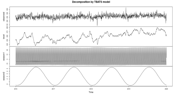
To improve understanding of the time series, I applied a TBATS decomposition to the data. Other more common decomposition methods such as X11 could not be used as they do not handle multiple seasonality.
Figure 10: TBATS decomposition of the daily number of attendances at the A&E from the beginning of 2016 to the end of 2019.
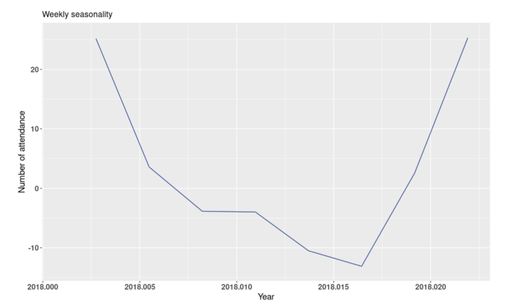
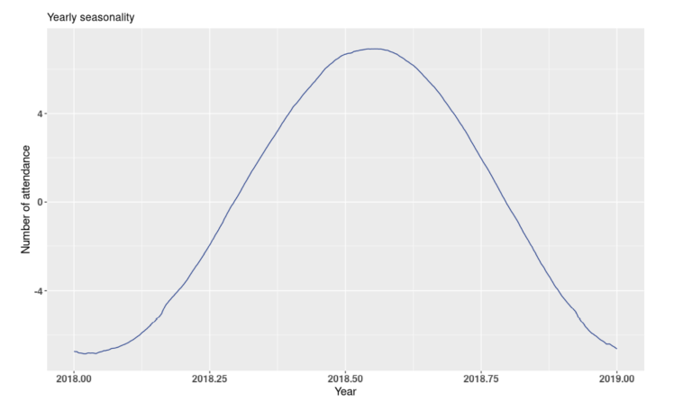
In figure 10, the first plot corresponds to the actual daily attendances at the A&E. The second plot represents the level of the time series, which roughly corresponds to the trend. The third and fourth plots represent the weekly and yearly seasonality, respectively. From figure 11, we can see that the TBATS model has successfully captured the weekly seasonality. There are 8 points in that plot corresponding to 8 days, with the first point being a Monday. Mondays’ average higher number of attendances is well represented. The yearly seasonality is also well captured in figure 12, where the summer months have on average a higher number of attendances.
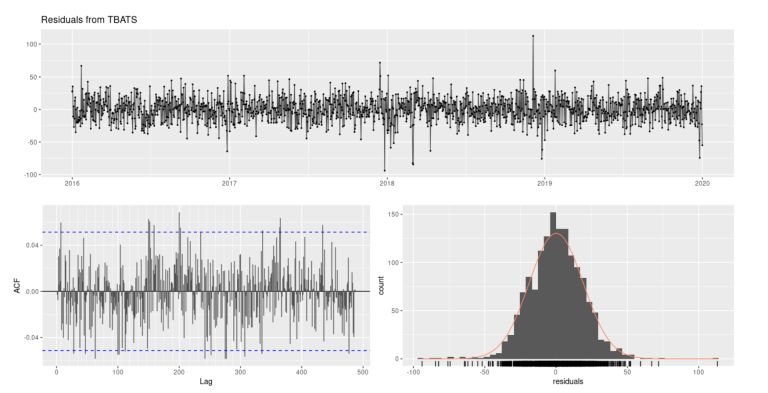
Next, we can apply several tests to ensure the residuals of the model resembled white noise. The residuals from the TBATS look to have mean zero and are normally distributed (Fig.13). The ACF plot of residuals does not show any significant autocorrelation and the histogram of residuals are centred around zero and normally distributed. Additionally, performing a Ljung-Box test yields a p-value of 0.2457 which is greater than 0.05. Therefore, we can assume that residuals are independent. Thus, all non-randomness has been well captured by the model.
Figure 13: TBATS residuals plot (Top), ACF of residuals (Bottom left), Histogram of residuals (Bottom right).
3 Forecasting daily attendances, results and limitations.
In this section, three different models which account for multiple seasonalities will be used to forecast the average daily number of attendances at A&E. The two seasonalities of the time series have length 365.25 and 7 days. The time series shows a positive trend and an additive seasonal pattern. The data was split 80/20 into a training dataset (1169 days) and a testing dataset (292 days). The first model we will look at is the TBATS (Trigonometric, Box-Cox transformation, ARMA errors, Trend, Seasonal components) model. The second model is an ARIMA model with Fourier series as external regressor. Finally the third model is an Autoregressive Neural Network model. We will then look at combining the different models to try and improve our predictive accuracy.
3.1 Forecasting using TBATS
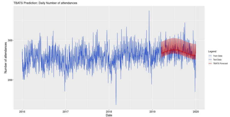
Figure 14 shows the daily number of attendances at the A&E, from January 2016 to the end of 2019. The blue line corresponds to the actual data and was split 80/20 between training and testing, respectively. The red line corresponds to the TBATS forecasts from March 15th, 2019 to December 31st, 2019. The TBATS forecast and testing datasets have equal length (292 daily figures).
Figure 14: Daily number of attendances from 2016 to the end of 2019 and TBATS forecast from March 15th, 2019 to the end of 2019.
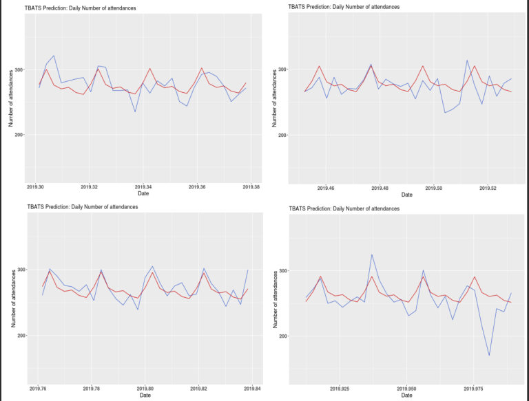
From figure 15, the TBATS forecasts look to be reasonably close to the actual daily number of attendances. However, the TBATS model struggles to predict spikes in the data, especially negative ones.
Figure 15: Four 4 weeks plots of daily number of attendances at A&E, TBATS forecast (red) and test data (blue).
3.2 Forecasting using ARIMA model and Fourier series as external
regressor
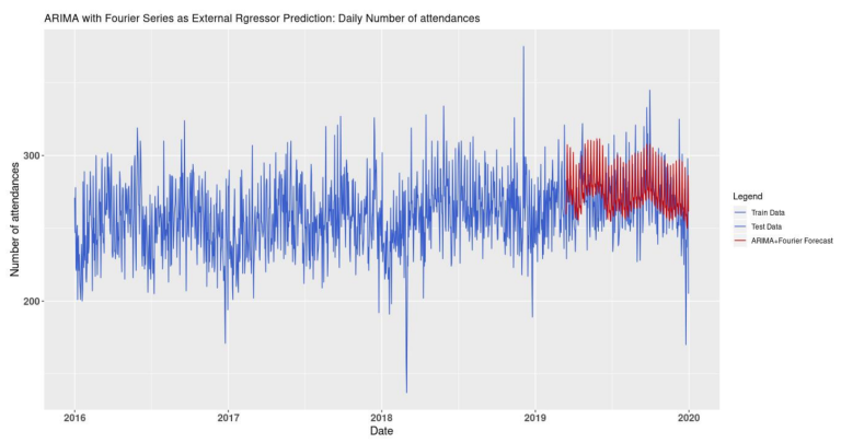
In order to select the optimal number of Fourier terms for each seasonality, two nested for loops were created to identify the number of terms which minimises the AIC. According to the algorithm, 3 and 10 terms are optimal for the weekly and yearly seasonalities, respectively. Figure 16 shows the actual daily number of attendances at the A&E (blue line) and the ones forecasted by the ARIMA model with Fourier series as external regressor (red line).
Figure 16: Daily number of attendances from 2016 to the end of 2019 and ARIMA with Fourier series as external regressor forecast from March 15th, 2019 to the end of 2019.
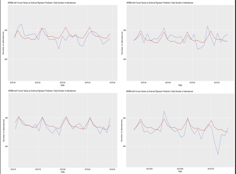
As shown in figure 17, the forecasted figures look reasonably close to the actual data. However, similarly to the TBATS forecasts, the negative spikes in the data are not predicted very well.
Figure 17: Four 4 weeks plots of daily number of attendances at A&E, ARIMA with Fourier series as external regressor forecast (red) and test data (blue).
3.3 Forecasting with an Autoregressive Neural Network model
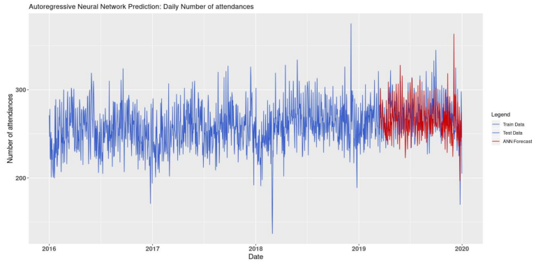
Looking at figure 18, we can see that the autoregressive neural network forecasts seem relatively close to the actual data. Furthermore, it appears to be able to predict some spikes in the data.
Figure 18: Daily number of attendances from 2016 to the end of 2019 and Autoregressive Neural Network forecast from March 15th, 2019 to the end of 2019.
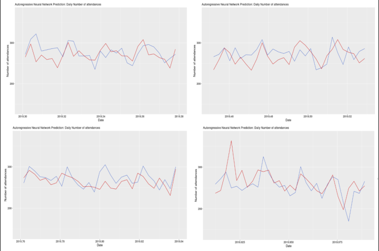
The autoregressive neural network (ANN) does not look to have captured the seasonality of the time series as well as the other two models. However, it seems better at predicting spikes in the data. When forecasting the daily number of attendances at the A&E using the autoregressive neural network, I tested if forecasts based on detrended and deseasonalised data would yield a more accurate prediction. This revealed that detrending and deseasonalising the data did increase the forecast’s accuracy (results are shown in the Results and Limitations section below).
Figure 19: Four 4 weeks plots of daily number of attendances at A&E, Autoregressive Neural Network (red) and test data (blue).
3.4 Combining forecasting models
It is sometimes possible to improve the forecasts’ accuracy by combining predictions from different models. The forecasts from the three models tested above were combined using two different methods. The first method consisted of using an aggregation algorithm (here a Polynomial Potential aggregation) which would decide the weights used when combining the daily number of attendances from the different forecasts. The weights were assigned as to minimise the loss function (here the mean square error). This was done for all possible combinations of the three forecasts using the function mixture() from the package ‘opera’. The second method used to combine the forecasts was to average the daily predictions. This was also done for all possible combinations of the three forecasts.
3.5 Results and Limitations
I used two different accuracy measures to compare the forecasts. First, the Mean Absolute Error (MAE) gives the average number of attendances by which the forecasts and the actual data differ across the 292 days forecasted. Secondly, the Root Mean Squared Error (RMSE) which computes the square root of the mean of the squared residuals. These two measures were obtained comparing the 292 daily number of attendances from the test data and the forecasts. Both MAE and RMSE are scale dependant which implies that they can be used to compare forecasts made on the same dataset.
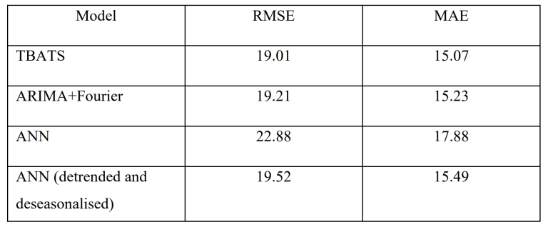
Table 2 shows that detrending and deseasonalizing the ANN increased the accuracy of the forecast. The RMSE and the MAE both reduced, from 22.88 to 19.52 and 17.88 to 15.49, respectively. However, it is the TBATS model which produced the most accurate forecasts with a RMSE of 19.01 and a MAE of 15.07.
Table 2: RMSE and MAE from the forecasts of 292 daily number of attendances at A&E, from March 15th, 2019 to the end of 2019.
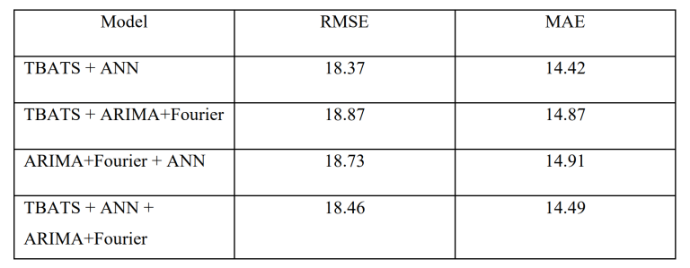
Combining forecasts reduced the RMSE and MAE for all prediction combinations when using the aggregation algorithm which minimises the mean square error. The most accurate forecast was obtained when combining the predictions from the TBATS model and the ANN. The forecast of this combination produced a RMSE of 18.37 and a MAE of 14.42 (Tab.3). Moreover, the predictions made from averaging the forecasts yielded mixed results. Only predictions made from combining all three forecasts or combining TBATS and ANN were more accurate than the forecasts made by the models separately.
Table 3: RMSE and MAE from combined forecasts (using an aggregation algorithm) of 292 daily number of attendances at A&E, from March 15th, 2019 to the end of 2019.
Nevertheless, there are three major limitations to the forecasts produced above. 1) The forecasts are based only on past observations and no other variables are used in the predictions. This limits how accurate the forecasts can be. To improve the forecasts, other variables should be accounted for such as weather (potential increase in car accidents on very rainy day) or festive periods (around Christmas more people get injured due to increase alcohol consumption, installation of decorations and time spent in the kitchen). 2) The models cannot forecast significant changes in the number of attendances and therefore cannot predict strong spikes in the data. 3) Finally, if the recording guidelines of what is considered an attendance and/or the A&E’s capacity change (such as an extension is built), then the current forecasts will need to be revised.
However, forecasting the daily average number of attendances at A&E departments can help hospitals. It can provide guidance on the amount of stock which needs to be purchased. It can help decide how many new staff need to be recruited and how to schedule their shifts. Overall, it will improve the quality of service and reduce the patients’ waiting time.