Gaussian Processes in Regression

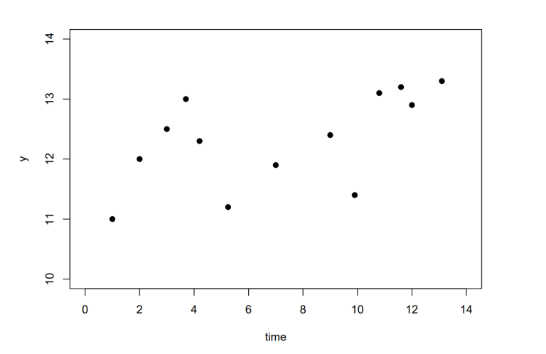
Lets assume we are interested in making predictions, based on a set of data points represented in Figure 1. Naturally, if we want to make predictions for a specific value $x_*$ where $x$ is a continuous variable, then it is very unlikely to have already made an observation for this new value $x_*$ . Thus, having discrete data is very limiting. Ideally, we would like to find a function, $f$ , which can be use instead of the discrete data to make predictions. Typically, this can be done in several different ways but one of them introduces Gaussian Processes in the context of regression. To obtain the desired function $f$ which goes through all of our observed data points, we attribute a prior probability to every possible functions, reflecting how likely we believe they are to best represent our data. It is immediately obvious that assigning a prior probability to the infinite number of existing functions is a major limitation, as it would potentially require an infinite amount of time. This problem is solved by Gaussian Processes which can be used as a prior probability distribution over all the functions. Inference in the GP made on a finite subset of the function f while ignoring the infinite number of remaining points will produce the same solution as if we had accounted for them (Williams & Rasmussen 2006).

Definition (Gaussian Process)

A Gaussian Process is a collection of random variables (indexed by time or space), of which, any finite number have a joint Gaussian distribution (i.e. multivariate normal distribution).

We denote a GP as follows:

$f(\boldsymbol{x}) \ \sim \ \mathcal{GP}(m(\boldsymbol{x}), k(\boldsymbol{x}, \boldsymbol{x'})),$ (1)

where,

$\boldsymbol{x}$ and $\boldsymbol{x^'}$ , are input vectors of dimension $D$ ,
$m(\boldsymbol{x})$ , is the mean function,
$k(\boldsymbol{x,x^'})$ , is the covariance function also know as the kernel.

Therefore, a GP is completely specified by its mean function and kernel, corresponding to Equation (2) and (3) respectively. However, it is common to set the mean function to be zero and de-mean the data. This is done to simplify the model and works well if interested only in the local behaviour of our model.

$m(\boldsymbol{x}) = \mathbb{E}[f(\boldsymbol{x})],$ (2)

$k(\boldsymbol{x}, \boldsymbol{x'}) = \mathbb{E}[(f(\boldsymbol{x})-m(\boldsymbol{x}))(f(\boldsymbol{x'})-m(\boldsymbol{x'}))].$ (3)

Generally, the covariance function chosen will contain some free parameters which in the context of GP’s are referred to as hyperparameters. Hyperparameters have a very strong influence on the predictions from our GP. Graphically, they define the ‘shape’ of our GP and control the level of fitting to the data. There exist many different covariance functions and the methods used to choose the right one are discussed in Section 4. The hyperparameters for the squared-exponential covariance function (Equation (4)) are the signal variance $\sigma^2_f$ , the length-scale $l$ and the noise variance $\sigma^2_n$ .

$k(x_a,x_b)=\sigma^2_{f}\exp{(-\frac{1}{2l^2}}(x_a – x_b)^2)+\sigma^2_{n}\mathbb{I}.$ (4)

This is one of the most commonly used covariance function as samples from a GP with squared-exponential covariance function will be continuous and infinitely differentiable. Continuity produces smooth curves which makes it easy to interpret the results and the infinite differentiability is useful to integrate prior knowledge about likely values of the derivatives.

GPs are interesting because of their marginalisation property. This property means the distribution of the existing data will not be affected by the addition of new data points. For example, if the GP specifies $(z_1, z_2) \sim \mathcal{N}(\boldsymbol{\mu}, \Sigma)$ then $z_1 \sim \mathcal{N}(\mu_1, \Sigma_{1,1})$ where $\Sigma_{1,1}$ where $\Sigma_{1,1}$ is the relevant submatrix of $\Sigma$ . Given a chosen covariance function, we can now produce a random Gaussian vector, where, $X_*$ , is a $D \times n$ matrix of tests inputs and $K$ , is the covariance function,

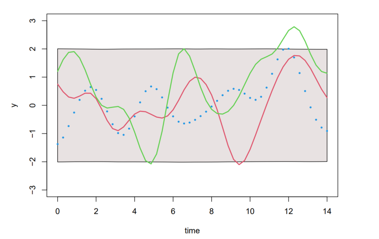
$\textbf{ f}_{*} \ \sim \ \mathcal{N}(\boldsymbol{0}, K(X_*,X_*)).$ (5)

Throughout this paper, the bold lowercase notation $x$ represents a special case of $X$ for dimension $D \times 1$ , the corresponding covariance functions are written as $k$ and $K$ for $x$ and $X$ , respectively. Similarly, the subscript “ ∗ ” indicates test inputs (i.e. the indices of the unobserved values we are trying to predict). Figure 2 shows three such samples generated by Equation (5), these are functions drawn randomly from a GP prior.

Next, we would also like to account for the information given by the observed data points (e.g. the data in Figure 1). This can be done using the joint distribution of the training output $f$ and the test outputs $f _*$ , given by:

$\begin{bmatrix} \textbf{f} \\ \textbf{f}_{*} \end{bmatrix} \ \sim \ \mathcal{N}\Bigg(\boldsymbol{0}, \begin{bmatrix} K(X,X) & K(X,X_*) \\ K(X_*,X) & K(X_*,X_*) \end{bmatrix}\Bigg).$ (6)

Although, this assumes that our observed values are noise free. In practice it is more realistic to assume some white noise exist. Writting it as $y = f(x) + ϵ$ , the joint distribution of the observed target values and the function values at the chosen test locations is now:

$\begin{bmatrix} \textbf{y} \\ \textbf{f}_{*} \end{bmatrix} \ \sim \ \mathcal{N}\Bigg(\boldsymbol{0}, \begin{bmatrix} K(X,X) + \sigma_{n}^{2}\mathbb{I} & K(X,X_*) \\ K(X_*,X) & K(X_*,X_*) \end{bmatrix}\Bigg).$ (7)

Here, $K(X, X*)$ is a $n \times n_*$ matrix for the n training points and $n_*$ chosen test points.

We can finally obtain the posterior distribution over all functions which go through the data points observed. Instead of checking the functions one by one, the conditional joint Gaussian prior distribution on the observed data can be used. This is done by sampling the function values $f_*$ from the joint posterior distribution by evaluating the mean and covariance matrix from:

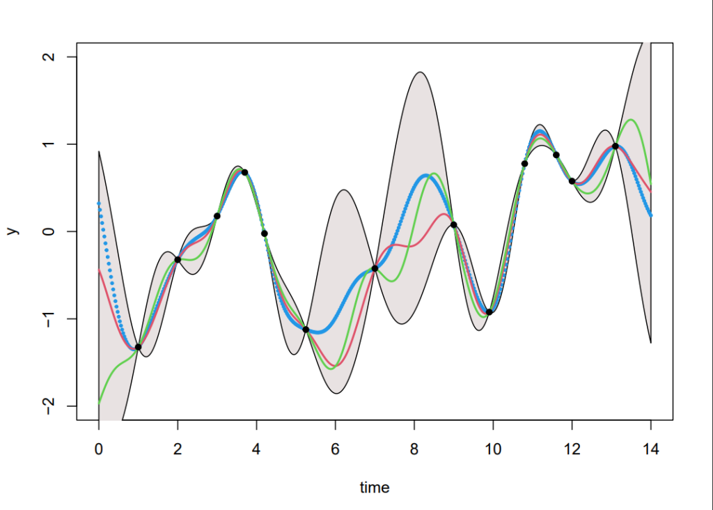
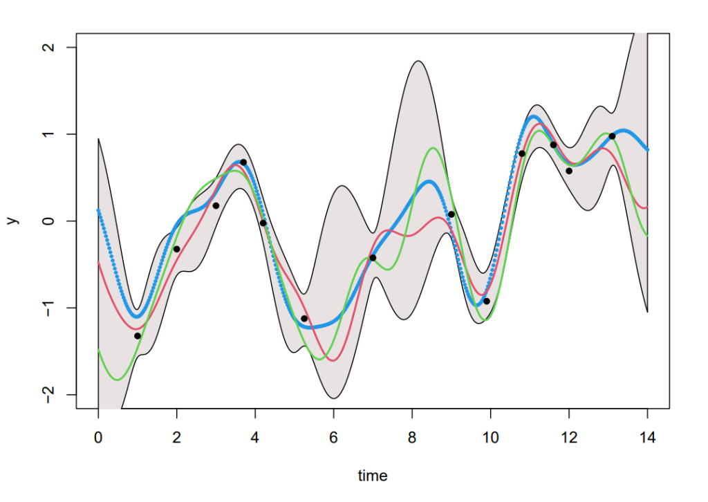
$\textbf{f}_* | X_{*}, X, \boldsymbol{y} \sim \mathcal{N}\big(K(X_{*},X) [K(X,X)+\sigma_{n}^{2}\mathbb{I}]^{-1}\boldsymbol{y}, K(X_{*},X_{*})-K(X_{*},X)[K(X,X)+\sigma_{n}^{2}\mathbb{I}]^{-1}K(X,X_{*})\big).$ (8)

Generating samples from Equation (8), we can produce Figure 3. Although this is straight forward in theory, in practice an additional step using Cholesky factorisation was included to avoid numerical instabilities from inverting the kernels (see code in Section 8). The coloured functions are directly sampled from the posterior whereas the grey areas are obtained by calculating the pointwise mean of all the sampled functions plus and minus twice the standard deviation for each input value (this corresponds a 95% confidence region).