Hi! As you know I have started my first year of PhD, and my research direction is anomaly detection. And it could be seen as some special changepoint questions. So I started to write some notes during my PhD learning period. This is suitable for people already familiar with changepoint algorithms and who wants to have a look. I am happy to discuss with you my notes if there is something I misunderstand:)
To detect the change!
The story begins by detecting the change. Assume we observed data from time \( 1 \) to time \( t \) ; we could name this sequence of observations by \( y_1, y_2,…, y_t \). We aim to infer the locations and numbers of these changes – that is, to infer \( \tau \) . This question could be easily transferred to a classification problem, that is, how could we classify an ordered sequence into several categories as good as we can. Based on this idea, we could write the following minimisation problem:
$$ \min_{K \in N ; \tau_1,\tau_2,…,\tau_K} \sum_{k=0}^K L(y_{\tau_k+1:\tau_{k+1}}), $$
\( L(y_{\tau_k+1:\tau_{k+1}})\) represents the cost for modelling the data \( y_{\tau_k+1},y_{\tau_k+2},…,y_{\tau_{k+1}} \) as a segment, it could be the negative log-likelihood; \( K \) is the total number of changepoints. Thus, this problem means we want to classify the ordered sequence into \( K+1 \) segments and make sure the classification could achieve the minimum log-likelihood. A question is that if we directly use this minimisation expression, we will always assign only one observation into one segment. Imagine that if we have 3 data points, when \( K=2 \) , we always achieve its minimum coz the cost for each segment is 0 and the sum is 0 too. Thus, we need a constrain!
Constrained problem and penalised optimisation problem
If we know the optimal number of changepoint \( K \) , we could force our algorithm to find \( K+1 \) segments. This is the constrained problem:
$$Q_n^K=\min_{K \in N ; \tau_1,\tau_2,…,\tau_K} \sum_{k=0}^K L(y_{\tau_k+1:\tau_{k+1}}), $$
Solve the RHS of the above equation by dynamic programming; we will get the optimal location of \( K \) changepoints. However, this requires prior knowledge of the number of changepoints. When we don’t know the exact number of changepoint, we could try to give a maximum number of changepoints, e.g.10; then compute \( Q_n^k \) for all \( k=0,1,2,…,10 \) , and choose the minimum \( Q_n^k \) as the final solution. In general, it could be written like:
$$\min_k[Q_n^k+g(k,n)],$$
where \( g(k,n) \) is the penalty function for overfitting the number of changepoints.
Given this idea above, a group of clever people think why not transfer the problem into a penalised one. If the penalty function is linear in \( k \) , say, \( g(k,n)=\beta k, \beta>0 \), we could write it as:
$$Q_{n,\beta}=\min_{k}[Q_n^k+\beta k]=\min_{k,\tau}[\sum_{k=0}^K L(y_{\tau_k+1:\tau_{k+1}})+\beta ] – \beta$$
This is known as the penalised optimisation problem. And all our stories come from here.
To solve the penalised optimisation problem, we could use dynamic programming! Given \( Q_{0,\beta}=-\beta \) , we have
$$Q_{t,\beta}=\min_{0\leq\tau<t} [Q_{\tau,\beta}+L(y_{\tau+1:t})+\beta],$$
for \( t=1,2,…,n \) . However, solving this one requires \( O(n^2) \) time complexity! Because of each step, we have to recalculate the cost for each observation. In order to reduce the computational complexity, two approaches have been proposed – PELT and FPOP!
PELT
Let’s look at some maths first! Assume there exists a constant $a$ and
$$Q_\tau + L(y_{\tau+1:t}) +a >Q_t,$$
\( y_\tau \) will never be the optimal change point in the future recursion. The LHS of the inequality above means the cost for modelling data have a changepoint at \( \tau \) until time \( t \) , while the RHS represents the cost without changepoint at \( \tau \) . Thus, in the following calculation, we do not need to consider the possibility that $\tau$ is the optimal last changepoint. So, the search space is reduced!
In each recursion, instead of calculating the cost and finding the minimum, we need to add an additional step to check if the inequality holds. In the worst cases, the computational complexity is still \( O(n^2) \) . However, when the number of changepoint increases with the number of observations, PELT could achieve linear computational complexity!
FPOP
FPOP is functional pruning. In the optimisation problem, we firstly model the segment then find the minimisation. But functional pruning swaps the order of minimisation, that is to find the segment for different parameters. Assume cost function could be represented as the sum of \( \gamma(y_i,\theta), \) you will be very clear if we do some maths:
$$\begin{split} Q_t&=\min_{0 \leq \tau < t} [Q_\tau+L(y_{\tau+1:t})+\beta]\\&=\min_{0 \leq \tau < t} [Q_\tau+\min_\theta \sum_{i=\tau+1}^t \gamma(y_{i,\theta})+\beta]\;\;\;\; (\mathrm{independent\; assumption})\\&=\min_{\theta} \min_{0 \leq \tau < t} [Q_\tau+\sum_{i=\tau+1}^t \gamma(y_{i,\theta})+\beta]\\& = \min_{\theta} \min_{0 \leq \tau < t} q_t^\tau(\theta)\\&=\min_{\theta} Q_t(\theta),\end{split} $$
where \( q_t^\tau(\theta) \) is the optimal cost of partitioning the data up to time \( t \) conditional on the last changepoint being at \( \tau \) with the current parameter being \( \theta \) ; and \( Q_t(\theta) \) is the optimal cost of partitioning the data up to time \( t \) with the current segment parameter being \( \theta \) . Simply, assume we have two possible changepoint candidates \( \tau_1 \) and \( \tau_2 \) , \( \tau_1 \) will never be the optimal partition if \( q^{\tau_1}_t > q^{\tau_2}_t \) , then we could simply prune \( \tau_1 \) .
You could easily find the difference. Before in penalised optimisation problem, we firstly find the possible partition and then estimate the parameter in the segment, and then find the minimum cost. As a result, the associated partition is the solution we want. But here, we have possible estimated parameters, for each estimated parameter, we have corresponded partition. Then the minimum cost over all possible parameters is the solution we want.
The equation above could be easily solved by dynamic programming:
$$Q_t(\theta)=\min \big\{Q_{t-1}(\theta), \min_\theta Q_{t-1}(\theta)+\beta\big\}+\gamma(y_t,\theta)$$
The former one in the bracket means there is no new changepoint in the last iteration, while the latter one in the bracket means that add a new changepoint in the last iteration after updating one observation. In the worst case, the time complexity is \( O(n^2) \) ; but in the best case, the time complexity is \( O(n\log n) \) .
I will explain the Figure here, and you will understand how FPOP prune candidate changepoint.
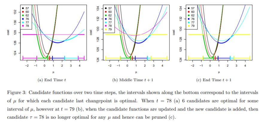
At time \( t=78 \) , we stored \( 7 \) intervals with associated \( \mu \) . Since we assume \( \gamma \) function is a negative loglikelihood for normally distributed data, it shows a quadratic shape in the Figure. At time \( t=79 \) , we observed new data, so we recompute the cost function and get the result as the middle Figure shows. In the middle Figure, notice that the purple line is not optimal anymore (it is above all the curves), and the purple line corresponds to the cost when the changepoint is located in 78. Thus, we could prune this candidate that we will not consider \( y_{78} \) to be the possible changepoint anymore (as shown in Figure (c)).