Spectral Synchronicity in the Human Brain – Part 1

The human brain is arguably one of the most complex structures ever to exist, consisting of around 86 billion neurons on average. Electrical activity in the brain is often the result of highly coordinated responses from a large number of neurons, both locally, within each brain region, and globally, across different regions. In this blog post, we investigate brain activity using Electroencephalograms (EEGs), which capture the oscillations produced by the coordinated activity of neurons.

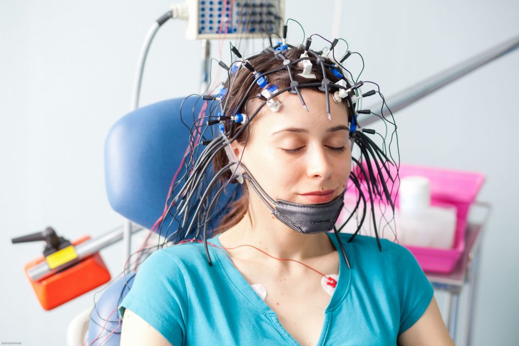
An EEG is a medical test during which small electrodes are attached to the scalp (see Figure 1 below). These electrodes detect electrical charges that result from neuronal activity. Importantly, EEGs can be used to help diagnose and monitor a number of conditions affecting the brain, including epilepsy.

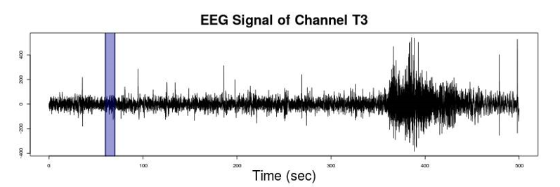
Figure 1: Visual representation of subject receiving an EEG test.

Statistically, EEGs are multivariate time series recordings that can be viewed as mixtures of oscillations with differing amplitudes across locations on the scalp. That is, we can denote by $X(t), t=1,\dots, T$ an EEG recording for one epoch at a single channel. Recall that a channel simply corresponds to the place at which an electrode is attached to the scalp. In the discussion that follows, we assume that the time series $X(t)$ is weakly stationary.

Figure 2 provides a visual exemplification of what an EEG recording at a given channel may look like. Highlighted in blue is a particular segment of the time series, this is what we refer to as an epoch in the paragraph above.

Figure 2: Visual representation of an EEG recording at a given channel.

The Spectral Density

When looking at EEG recordings, we are often interested in determining their oscillatory content. This can be achieved by estimating the spectral density. In short, the spectral density is capable of characterising the oscillatory content of the EEG, and describes the distribution of the total variance (energy) across all frequencies.

As you may have deduced from the previous paragraph, the spectral density is a concept specific to the frequency domain of time series analysis. For an introduction to the area, with specific content relating to the modelling of EEG recordings, I recommend Chapter 20 of the Handbook of Neuroimaging Data analysis.

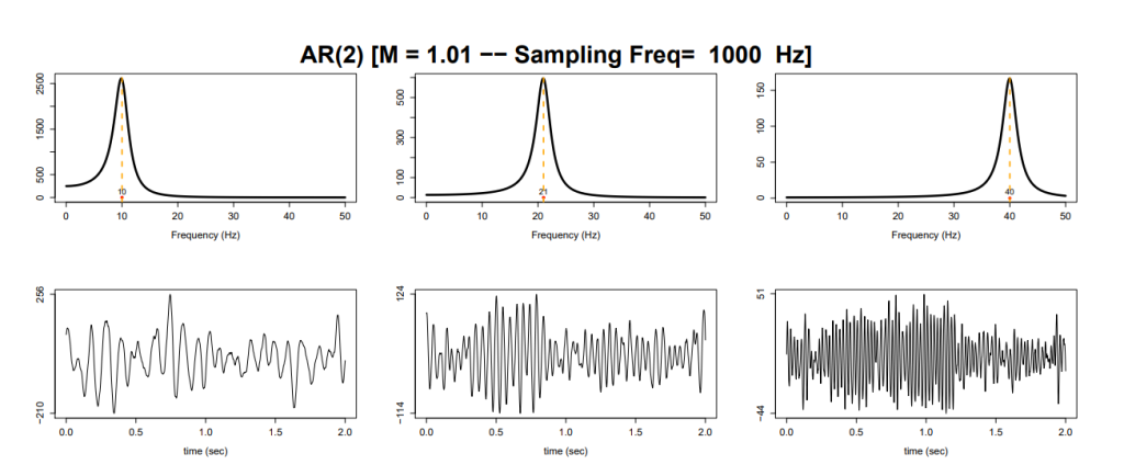
Rather than getting bogged down with the theory of spectral analysis, I have chosen to present a simple motivating example using an AR(2) process. The intended purpose of which is to demonstrate how the spectral density relates to the signal observed in the time domain.

Below are 3 realisations from an AR(2) process, each with spectral densities concentrated at different frequencies – namely 10Hz, 20Hz and 40Hz. Crucially, we see that time series with spectral densities concentrated around higher frequency values exhibit faster oscillations of the signal in the time domain, compared to those with spectral densities concentrated at lower frequencies.

Figure 3: Top: Spectral densities for AR(2) process concentrated at different frequencies. Bottom: Realisations from the corresponding AR(2) process.

The Hierarchical Spectral Merger Algorithm

Following on from my admittedly brief discussion of the spectral density, I now wish to discuss a way in which it can be used to identify a modular structure within the brain. More specifically, I am going to give a high level overview of a method called the Hierarchical Spectral Merger Algorithm (HSM).

Put simply, this algorithm is a clustering technique, and the overall idea is to construct clusters of brain signals that “co-activate” in the frequency domain. That is, assuming that the spectral density encapsulates all the information regarding the signal recorded at each channel, the HSM algorithm will construct clusters of channels that have similar spectral densities.

Total Variation Distance (TVD)

As is the case for any clustering approach, we first need to identify a way in which to measure similarity between the objects of interest. As aforementioned, the spectral density is the key feature on which we base our classification. Therefore, we are interested in measuring the similarity between spectral densities. This is achieved via the total variation distance (TVD).

We motivate the idea of TVD by considering two probability densities (see Figure 4 below). The main idea is to measure how similar two densities are by considering the common area below both densities, as depicted by the shaded region in Figure 4.

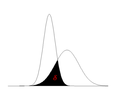
Figure 4: Graphical Representation of TVD. The shaded area is representative of the common area below both densities, denoted δ.

If we let this shaded region be denoted by $\delta$ , then the TVD can be defined as

$d_{TV} = 1 - \delta$ .

A desirable property of TVD as a similarity measure is that it is bounded on the interval [0, 1]. Consequently, the values obtained by this similarity measure are highly intuitive. More specifically, a value near 0 indicates that the densities are similar while a value near 1 indicates they are highly dissimilar.

The HSM Algorithm

Now that we have defined our measure of similarity between spectral densities, we are ready to introduce the HSM algorithm itself. We begin by setting up some necessary notation.

Let $X_c = [X_c(1), \dots, X_c(T)]$ be the EEG recording at channel $c, c = 1, \dots, N.$ The algorithm starts with a total of $N$ clusters representative of the $N$ unique channels. The iterative steps of the algorithm are listed below.

Suppose there are $k$ clusters. Estimate the spectral density for each cluster, and represent each cluster by a common normalised spectral density denoted by $\hat{f}_j(\omega),$ where $\\ j=1,\dots, k.$
Compute the TVD between each pair of $k$ spectral densities.
Identify the 2 clusters that have the smallest TVD (save this value).
Merge the time series in the 2 clusters with the smallest TVD. We will use this single combined cluster in subsequent steps.
Repeat steps 1 to 4 until there is only 1 cluster.

The first step of the algorithm involves estimating the spectral density for each EEG using something known as the smoothed periodogram. Many methods of estimation exist, however these are out with the scope of this blog post. If you are interested in finding out more about these estimators, then please see the further reading section below. Estimating the common spectral density used in subsequent repetitions of the algorithm (i.e. step 5 onwards) involves taking the weighted average over all the estimated spectral densities for each signal in the new cluster. This is highly intuitive since computing a new common spectral density will combine information across all the channels in a cluster, and thus will improve the quality of the spectral estimates.