This blog will give you the idea of choosing an appropriate statistical correlation test in social science area.
Recently I am talking with friends who are studying in the social science area, and they are confused about how to use statistical test appropriately. So I decided to write a series of blogs talking about the common statistical method in social science and how to explain the result.
In social science, it is common to calculate the association between two variables. For example, you may want to test the relationship between smoking and lung cancer, consumption and income, etc. The test method could be summarized in the table below under different variables and different distributions. In this blog, we only measure two continuous variables.
| Two continuous variables | |
| Normal distributed? | Pearson Correlation coefficient |
| Not normal distributed | Spearman Correlation coefficient |
| Two categorical variables | Fisher exact test; Chi-square test |
| one continuous variable and one continuous variable | Boxplot; Biserial rank correlation |
Analysis of Correlation
Drawing the plot – a direct way
The first step of measuring the correlation is drawing the plot:
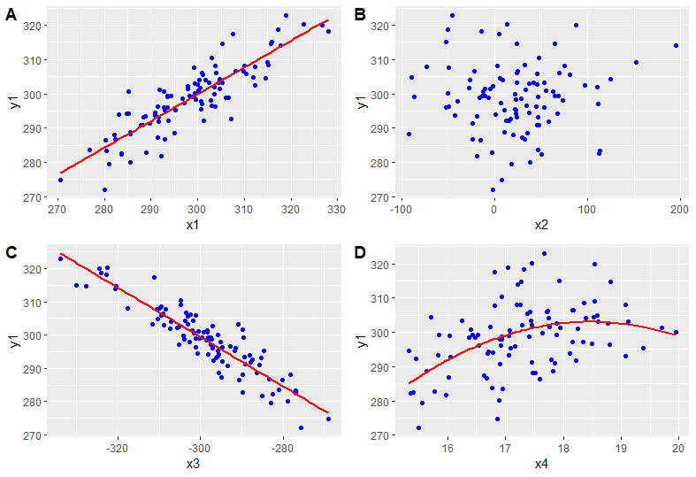
Assume we have continuous data y1, x1, x2, x3 and x4. From the plot above, we could see the correlation between y1 and x1 is a positive linear correlation; y2 and x2 seem no apparent linear correlation and non-linear correlation; y1 and x3 have negative linear correlation and y1 and x4 have a non-linear correlation.
Calculating the correlation coefficient – a mathematical way
The correlation coefficient is a statistic measuring the strength of the linear correlation. Usually, there are two ways: the Pearson correlation coefficient and the Spearman correlation coefficient. Although you may want to report the P-value of the correlation test, it is necessary to report the coefficient at the same time.
Pearson correlation coefficient
Pearson correlation coefficient could be calculated in R by cor() function. It is the most commonly used statistics; However, it assumes normal or bell-shaped distribution for continuous variable. We didn’t check the assumption here but it has to be done in real data analysis.
The correlation coefficient ranges from -1 to 1. The sign measures the direction of correlation: positive refers to the positive relationship while negative value refers to the negative relationship. The absolute value measures the strength of the correlation. Usually, the absolute value |value|>0.7 could be considered as a strong correlation.
From the example we could see, y1 and x1 have a strong positive correlation; the correlation coefficient between y1 and x2 is really small only 0.016; y1 and x3 have a strong negative correlation; while y1 and x4 have a mild correlation. Note: Here we could only say they have a linear correlation since Pearson ignore the non-linear relationship.
> cor(y1,x1)
[1] 0.8708785
> cor(y1,x2)
[1] 0.01631352
> cor(y1,x3)
[1] -0.9145617
> cor(y1,x4)
[1] 0.405236
Spearman Rank correlation coefficient
Unlike Pearson’s method, Spearman’s method does not assume the distribution of the variables. Usually, we got a similar result to Pearson (as the result we see below). The difference between the Spearman rank correlation and Pearson rank correlation is that Pearson only takes account into the linear relationship but discards non-linear relationship. However, the Spearman test considers both linear and non-linear relationship.
> cor(y1,x1,method = 'spearman')
[1] 0.8520012
> cor(y1,x2,method = 'spearman')
[1] 0.01749775
> cor(y1,x3,method = 'spearman')
[1] -0.9017702
> cor(y1,x4,method = 'spearman')
[1] 0.4252865
How we report?
- Firstly, draw the plot to see the relationship.
- If you want a statistical test:
- draw the histogram to see if they have a normal/bell-shaped distribution
- If yes, using a test with the Pearson method
- If no, using the test with the Spearman method
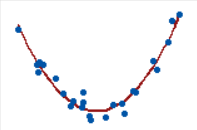
It is worth noting that the statistical test is only an assisted tool for the relationship plot. Since in some cases, the result of the test is not reliable. For example, we could see a strong nonlinear correlation in the plot below. However, the Pearson coefficient and Spearman coefficient are both approximately 0.
Besides, we could only say there is a correlation between variables and we could not get a conclusion that one variable is the causality of another variable. Specifically, if two variables have a large correlation of 0.9 and variable A has a high value, variable B will probably have a high value. However, we could not say high value in variable A causes the high value in variable B.
For more readings:
http://www.sthda.com/english/wiki/correlation-test-between-two-variables-in-r This blog specifically listed how to conduct other correlation test between two variables in R
https://www.statisticshowto.com/probability-and-statistics/correlation-coefficient-formula/ This is a really good blog about the definition and it also contains a good video!