In the early 1960s, the Soviet Union was giving their cold war enemies the USA a thrashing in the space race. In response, president John F. Kennedy decided to focus NASAs efforts on getting a human to set foot on the moon to try and score a big victory for the Americans.
This challenge was an appreciable step up from launching something into the Earth’s orbit. The NASA engineers needed to make their spacecraft closely follow a precisely calculated trajectory between the Earth and the Moon and then back again.
Making a spacecraft follow this trajectory runs into a few problems. Firstly, it is not just a simple case of plugging some numbers into equations of motion and then using the equations to predict the motion of the spacecraft. These equations make certain assumptions that are not followed in reality. They are a good guide but not precise enough. Secondly, the instruments installed on the spacecraft can only take measurements at irregular intervals and these measurements are subject to random noise. It is not just a case of taking measurements every millisecond and correcting for them.
This situation has the makings of a statistical problem, we have an underlying model of the spacecrafts position that is subject to random noise due to assumptions not being held and some sporadic and noisy measurements. From this information, we want to try and give the best estimate of the spacecrafts true position.
As luck would have it, one of the NASA engineers working on this problem Stanley F. Schmidt spoke to one of his old acquaintances, an electrical engineer named Rudolph Kalman, who had just published some mathematics that would enable just this kind of estimate.

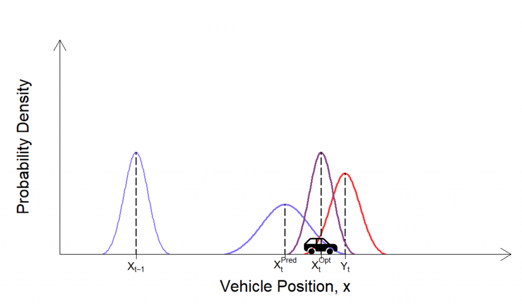
The idea behind the Kalman filter is illustrated by the simple example given in the figure above. The position of a vehicle is estimated by using the combination of a prediction made by using equations of motion (shown in blue) and a measurement (shown in red). These two components have a Gaussian shape due to the noise associated with them. The Kalman filter then takes a weighted average of the prediction and the measurement to give an optimal estimate of the position (shown in purple) which is more accurate and precise than both of the individual estimates. The weighting given to the prediction and measurement when the Kalman Filter calculates its estimate depends on which of the two the Kalman filter believes is more likely to be correct.
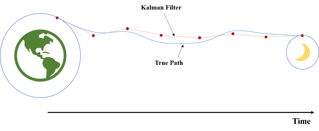
It was more or less, this simple realisation by Kalman that enabled Schmidt and his team to iron out a few wrinkles and develop a Kalman filter that was used on every Apollo lunar mission to give precise estimates of the spacecrafts position and enable the complex orbital trajectories essential to these missions. I’ve included a diagram here that simplifies the reality a little bit but you can imagine that the spacecraft is updating it’s Kalman filter estimate at points in time and then making adjustments to try and stay on the right path. Note that the true path of the ship differs slightly from the path the Kalman filter thinks it is taking. This is natural and isn’t a problem as long as these paths are similar enough. Also, the way the filter works means that these paths will become more similar over time.

Something I have overlooked so far is how the beautiful simplicity of the Kalman filter meant that it could be programmed on the Apollo computer that was orders of magnitude less powerful than a modern smartphone. All the Kalman filter needed to do was calculate the predicted position and record the measurement with onboard instruments at a given time to work out its optimal estimate. This could then just be repeated at each point in time by updating the previous estimate based on new information. i.e. in a recursive manner.
These days, the Kalman filter still finds applications in many tracking settings, GPS working in conjunction with the accelerometer and gyroscope in smartphones for example. It’s important to the development of future technologies such as self-driving cars and robotic workers. That’s not to say that the Kalman filter hasn’t undergone advances since the 1960s. These advancements have mainly been concerned with developing techniques that work well in which the relationship between the prediction made by the filter and its measurement are non-linear. An example of a more recent method that can tackle any problem in which there is non-linearity is the particle filter. The particle filter is a prime example of how far computing has came since man set foot on the moon as it never would have been possible to run the particle filter effectively using the computer on the Apollo spacecraft.
Relevant Links

