This blog will explain the one-way ANOVA test in detail (including assumptions, implementing situation and explanation), and an example analysed by R will be shown at the end.
What is this test for?
You may be familiar with the t-test and some other nonparametric test used to test if there is a difference in the mean between two groups (e.g., if there is a difference in mean score between two classes; if one treatment is better than another treatment). The one-way analysis of variance (ANOVA) is used to determine if there is a significant difference among the means of three or more independent groups. For example, the application situation could be:
- if there is a difference in mean score among the four classes
- if there is a difference in the mean effect among the three types of treatment
Assumptions:
There is no free lunch. To implement the one-way ANOVA test, it should satisfy three assumptions:
- The variable is normally distributed in each group in the one-way ANOVA (technically, it is the residuals that need to be normally distributed, but the results will be the same). For example, if we want to compare the mean score on three classes, the score should have a normal distribution for each class.
- The variances are homogenous. This means the population variance in each group should equal. For example, the scores of the students in the three classes should fluctuate by a similar level.
- The observations should be independent. This means one observation will not influence other observations. For example, student A’s grade will not influence student B’s grade as they took their exam independently.
All three test will be tested before implementing one-way ANOVA test. Now, let’s look at how to implementing ANOVA test through R.
How to do it and explain it (An example in R)
Let’s use the dataset in R called ‘PlantGrowth’. It includes the weight of 30 plants with three groups (10 plants will not receive any treatment (control group), 10 plants receive treatment A, and 10 plants receive treatment B). And our purpose is to find if there is a difference in the mean effect among the three groups?
Firstly, lets draw a boxplot to see the data graphically.
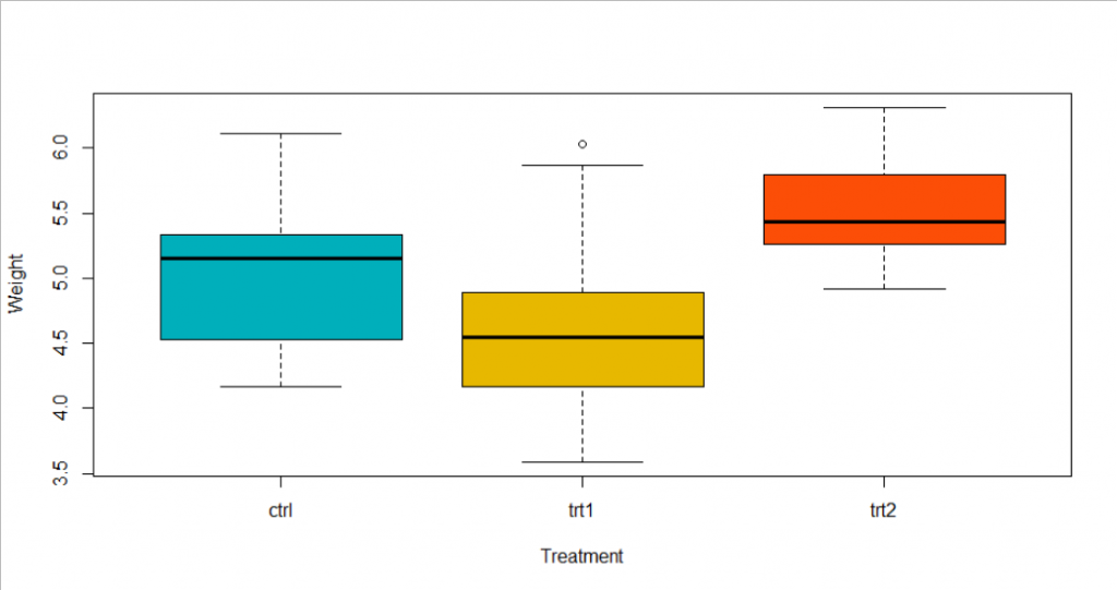
From the boxplot, we could conclude that treatment 1 has a lower effect than the control group, but the difference is not too large. And plants received treatment 3 has a larger weight than the other two groups.
Next, we measure the difference through One-way ANOVA, and we got the result:
res.aov <- aov(weight ~ group, data = data)
# Summary of the analysis
summary(res.aov)
            Df Sum Sq Mean Sq F value Pr(>F)
group        2  3.766  1.8832   4.846 0.0159 *
Residuals   27 10.492  0.3886
---
Signif. codes:  0 ‘***’ 0.001 ‘**’ 0.01 ‘*’ 0.05 ‘.’ 0.1 ‘ ’ 1
Interpretation
Under a 5% significance level, the P-value of the test is less than 0.05 (P=0.0159<0.05). So we could conclude there is a significant difference among groups.
However, we could only say there is a significant difference among groups, but we don’t know which pairs of groups are different. To understand if there is a difference between specific pairs of groups, we could implement Tukey multiple pairwise-comparisons:
TukeyHSD(res.aov)
  Tukey multiple comparisons of means
    95% family-wise confidence level
Fit: aov(formula = weight ~ group, data = data)
$group
            diff        lwr       upr     p adj
trt1-ctrl -0.371 -1.0622161 0.3202161 0.3908711
trt2-ctrl  0.494 -0.1972161 1.1852161 0.1979960
trt2-trt1  0.865  0.1737839 1.5562161 0.0120064
Under a 5% significance level, we could conclude that treatment 2 is significantly better than treatment1 on the mean weight of the plant. However, there is no statistical evidence that treatment 2 is better than treatment 1, and treatment 1 is worse than receiving no treatment.
Checking the assumptions
Now lets check the assumptions:
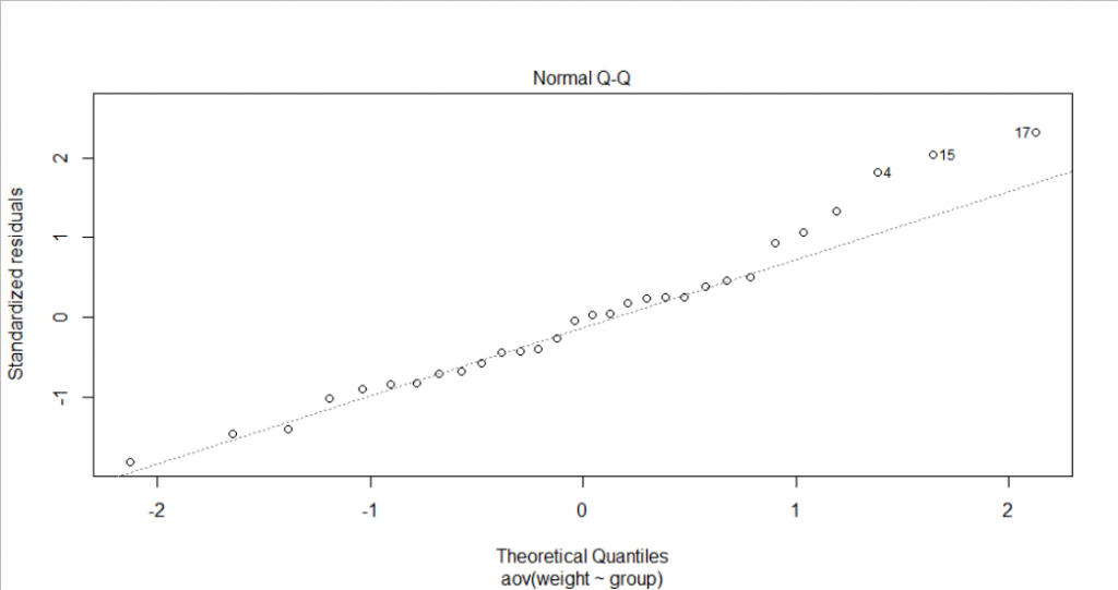
- Normally distributed assumptions. On the QQ plot, most points lie on the straight line except point 4, 15 and 17. However, we only have a small sample size (30 plants), so it is reasonable to see a normal QQ plot like this. We could also test the normality through the Shapiro-Wilk normality test. Under the 5% significance level, we could not reject the null hypothesis that the residuals are normally distributed.
shapiro.test(x = residuals(res.aov) )

	Shapiro-Wilk normality test

data:  residuals(res.aov)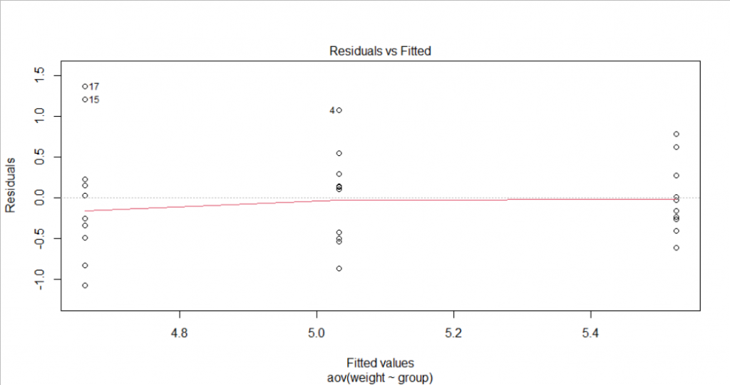
W = 0.96607, p-value = 0.4379- Homogenous variance assumption: From the Residual vs Fitted plot, we could see slight evidence of non-constant variance since the degree of dispersion for each group is different. However, it seems not serious. LeveneTest could also be done to test the homogeneity of variance. Under 5% significance, we could not reject the null hypothesis (P-value>0.05) to assume the homogeneity of variances in the different treatment groups.
leveneTest(weight ~ group, data =data)
Levene's Test for Homogeneity of Variance (center = median)
      Df F value Pr(>F)
group  2  1.1192 0.3412
27 - Independent assumption: This assumption needs more consideration. In our example, we could assume satisfying this independent assumption since the weight of one plant will not influence the weight of other plants.
That’s all done! This blog references the blog which including specific R code:
http://mathsbox.com/notebooks/python-utilities.html
Besides, I also found useful blogs which using SPSS to do one-way ANOVA test:
https://statistics.laerd.com/statistical-guides/one-way-anova-statistical-guide-3.php
https://statistics.laerd.com/spss-tutorials/one-way-anova-using-spss-statistics.php