For starters, what is Reinforcement Learning? When we learn in the real world, we are subconsciously aware of our surroundings and how they might respond to us when we take an action, the goal we wish to achieve via our actions, along with any repercussions our actions might have. Once we complete an action, we learn based on the consequences how effective our decisions were, and if necessary we adjust our actions for the future. In some sense, Reinforcement Learning hopes to replicate this more natural style of learning within a computational framework.
As a part of the MRes course we’re going off to dive into the Literature of an area we choose, with the aim to produce a longer report on the literature available. For me, this has been Reinforcement Learning. This will be the first in a series of posts for me to give a little bit of justice to the topic of RL.
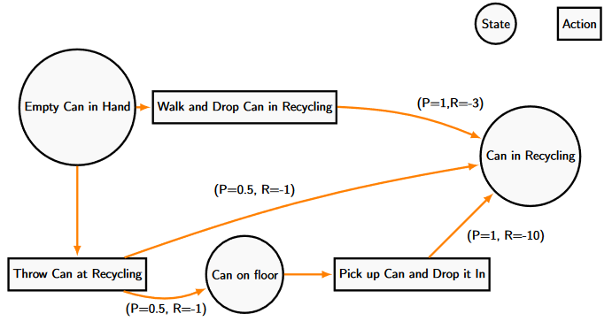
Let’s start with a little example I thought up while with a flatmate. If the goal is to recycle a can as fast as possible, one might simply walk over and place the can in the recycling. This option might be too slow for some people howevers, and alternatively one could throw the can at the recycling and hope it lands safely in the recycling bin. We are aware that while the second option could achieve the stated goal of correctly disposing of the can, and might save us a small amount of time, there exists the possible outcome in where the can lands somewhere on the floor. We then must gather up the item and place it into the recycling bin while groaning as your pasta secretly boils over in the background.
While not the most life-changing example, the Recycling example does show how many of the basic things we do in life are all made up of the same core parts as our Reinforcement Learning (And Markov Decision) Problems.
We begin with an agent (The human in the recycling example) that must be able to make decisions within the scenario and an environment which the agent must be able to interact with it. This environment includes various states that describe the conditions that the agent is in (the recycling example has three states, when the can in hand, in the recycling bin or somewhere on the floor). The state encompasses all of the information that is available to the agent at a given point in time. The must be a set of actions that the agent can take depending on the state they are in (the recycling agent can choose between throwing the can or carrying it), and there must be a reward signal that the agent receives after every action they take. The reward signal can be negative as to act as a disincentive for certain actions (as in the recycling example)
This all in all is the basic framework for Markov Decision Processes.
Markov Decision Processes (MDP) provide a classical formalisation for ordered decisions with stochastic components, and can be used to represent shortest path problems by constructing a general Markov decision problem. A Markov Decision Process relies on the notion of state, action, reward (just like above) and some transitional distribution for each action that describes how the agent moves between states. An MDP can be described as a controlled Markov chain, where the control is given at each step by the chosen action. The process then visits a sequence of states and can be evaluated through the observed rewards. Formally, we define the probability of transitioning between certain states, called the dynamics of the MDP, as the probability distribution:
\begin{equation}\label{dynamics}
p( s’, r | s , a ) = \mathcal{P}\{ S_t = s’, R_t = r | S_{t-1} = s, A_{t-1 = a}\} .
\end{equation}
This issue is, we generally are interested in the long term benefit we get from our actions rather than any short term benifit. We can then consider there to be some value function \(v(s)\) that describes the long term value being in a given state provides, which will let us navigate choosing an action in time. This value is generally given as the expected future reward \(R_{t+k+1}\) we will recieve after we’ve been in a state \(S_t=s\), discounted at each step by some fraction \( \gamma \). This just means that for each jump in time the value is less and less impactful the further and further away in time it is, called the State-value function, is given as
\begin{equation}\label{state-value}
v_{\pi}(s) = \textbf{E}_{\pi}[\sum_{k=0}^{\infty} \gamma^{k} R_{t+k+1}|S_t=s].
\end{equation}
There is similar motivation to define the value of any action \(a \in \mathcal{A} \) the agent might take while in state \(s\) following policy a decisions \(\pi\), hence we can define the value of the state-action pair following policy \(\pi\), \(q_{\pi}(s,a)\), called the Value-Action function as
\begin{equation}\label{action-value}
q_{\pi}(s,a) = \textbf{E}_{\pi}[\sum_{k=0}^{\infty} \gamma^{k} R_{t+k+1}|S_t=s, A_t = a].
\end{equation}
This brings us to the crux of MDPs. The true objective is to use our agent to find an optimal policy that maximises either \(v(s)\) or \(q(s,a)\). This is done by considering the Bellman Optimality Equations. This is the objective whe Solving MDPs, and almost all of traditional Reinfocement Learning is about estimating these state-value functions. The Bellman Optimality Equations highlight that if the agent is using an optimal policy, the value of a state must equal the expected return of the most valuable action from that state (if you’re doing the best then you’re making the best choices).The Bellman equations, which can be shown via some tomfoolery with the recursive nature of the Reward equation and the value equations, is given by
\begin{equation}\label{bell_v}
V_b(s) = max_\pi v(s) = max_a \sum_{s’,r} p( s’, r | s , a ) [r + \gamma V_b(s’)]
\end{equation}
or for the Action-Value function
\begin{equation}\label{bell_q}
q_b(s,a) = max_\pi q(s,a) = \sum_{s’,r} p( s’, r | s , a ) [r + \gamma max_{a’} q_b(s’,a’)].
\end{equation}
As any optimal policy would share both an optimal State-Value function and an Action-Value function, it is only necessary to solve one of the Bellman equations. For finite MDPs, the equations are guaranteed to have a unique solution that can be solved computationally as a set of non-linear equations, one for each state in the state space.
So while we have complete information on the problem, and while that state space isn’t too big, we can solve a set of non-linear equations to directly solve the MDP. However as you might expect, this isn’t always possible. Infact, for interesting problems this isn’t possible a lot of the time, so there is need in learning some estimate for these value equations… possibly through experience. See you the next post to talk about Reinforcement Learning proper! All the best,
– Jordan J Hood