As a part of our Masterclass lectures we were introduced to Splines and Functional Data Analysis, and as I came to realise how applicable Splines are to data analysis. Well why not take a dive into them?
Let’s say we have set of non-linear looking data that we wish to fit a model to. Splines can be seen as an extension to polynomial regression, where rather than fitting some high-degree polynomial function over the entire range of \(X\), we instead look to fit lower order, and more manageable, polynomials over smaller sub-regions within the range of \(X\), seperated by \(K\) total knots.
Knots are the points where we force our different polynomials to converge and have our coefficients change. For example if we had two knots located at points \(a\) and \(b\) respectively and a piecewise cubic polynomial, then the most basic structure we could have is
\begin{equation}
y_{i} =
\begin{cases}
\beta_{0,1}+\beta_{1,1} x_i+\beta_{2,1}x_i^2+\beta_{3,1} x_i^3 \text{ if } x_i < a \\
\beta_{0,2}+\beta_{1,2} x_i+\beta_{2,2} x_i^2+\beta_{3,2} x_i^3 \text{ if } a < x_i < b \\ \beta_{0,3} + \beta_{1,3} x_i + \beta_{2,3} x_i^2 + \beta_{3,3} x_i^3 \text{ if } b < x_i
\end{cases},
\end{equation}
although in general for basis functions \(\chi_p(x)\) and coefficients \(\beta_p\) we define the Basis-Expansion as
\begin{equation}
y(x) = \sum_{p=1}^{P}(\chi_p(x)\beta_p).
\end{equation}
Currently, however, these are not splines, just individually fitted cubics to the dataset. To fit a Spline, we also fix constraints at each knot. We force a constraint that at each know the polynomials are continuous, and we constrain both the 1st and 2nd derivatives to be continuous. This means the lowest order Spline that satisfies these requirements is the Cubic Spline, hence why they are so common! Although if we wish to investigate the derivatives of a model, such as for a chnage in weather or income, then we require a high order Spline than a Cubic.
In order to fit a Spline we perform least squares regression with \((K + O + 1)\) coefficients, where \(K\) is the number of knots and \(O\) is the order of the Spline (and 1 for the intercept). Hence fitting any cubic Spline consumes \((K+4)\) degrees of freedom. These are commonly called Regression Splines.
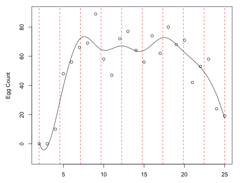
But how do we choose the Knots? Well there are few ways one might choose:
- Place even equally spaced Knots, such that we have some observations within each interval over the range of \(X\)
- Place a Knot at an every given amount of observations, so the area with the greatest number of observations has the most flexibility
- Place the Knots where there is the greatest variance in the observations
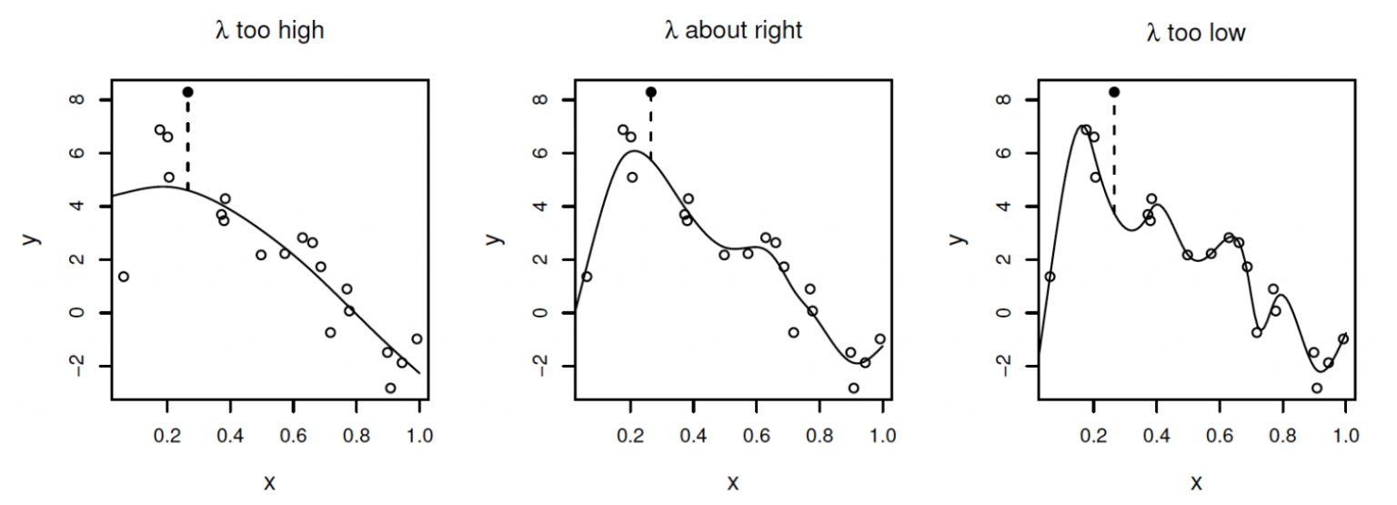
It should be highlighted that creating a set of Knots, generating basis functions and estimating coefficients via Least Squares isn’t the only way to use Splines. Moving on to Smoothing Splines, we’re now looking to fit a smooth curve of data, our objective is to find some function \(f(x)\) to fit as well as possible to our data, which we measure by minimising the Residual Sum of Squares. However we need to balance this between fitting the data and overfitting the data, as we could just draw a straight line between every point we observe in order, but that wouldn’t tell us anything! Hence we require our \(f(x)\) function to be smooth, while looking to minimise the RSS. Just as before, by smoothness we refer to a measure of the second derivative, and hence we now want to find the coefficients that minimise
\begin{equation}
\hat{\beta} = \min\left( \sum_{j=1}^{n}(y_j – y(x_j))^{2}+ \lambda \int\left[ \frac{d^{2}y(x)}{dx^{2}}\right]^{2} \right).
\end{equation}
Here we balance a fit to the data, \( \sum_{j=1}^{n}(y_j – y(x_j))^{2}\) with a smooth fit penalty \(\lambda \int \left[ \frac{d^{2}y(x)}{dx^{2}}\right]^{2} dx\), where in particular \(\lambda\) dictates how impactful the smooth penalty is.
From here, we can look at the Generalized Cross-Validation (GCV) score to give a prediction of the error in fit, choosing \(\lambda\) to minimise GCV. We can then move onto numerically estimating coefficient values and extending this methodoligy to forcibly fit our Splines to disributions by prior know behaviours. For example if you know the first or second order behaviour of your data, such as in many Ordinary Differential Equations. All the best,
– Jordan J Hood