So following up from the last post, we are looking to estimate the value of different states and actions or agent can take as part of some stochastic process. But how? By learning from experience. Trial and Error, over potentially thousands or millions of simuated episodes.
In particular there are two methods in Reinforcement Learning that will show up everywhere, Q-Learning and SARSA, and you cannot read an RL text without encountering either of them or any of their bigger better cousins. Frankly, it would be rude of me not to talk about them here.
Temporal Difference (TD) learning is likely the most core concept in Reinforcement Learning. Temporal Difference learning, as the name suggests, focuses on the differences the agent experiences in time. The methods aim to, for some policy (\ \pi \), provide and update some estimate \(V\) for the value of the policy \(v_{\pi}\) for all states or state-action pairs, updating as the agent experiences them.
The most basic method for TD learning is the TD(0) method. Temporal-Difference TD(0) learning updates the estimated value of a state \(V\) for policy based on the reward the agent received and the value of the state it transitioned to. Specifically, if our agent is in a current state \(s_{t}\), takes the action \(a_t\) and receives the reward \(r_t\), then we update our estimate of \(V\) following
\begin{equation}\label{TD0}
V(s_t) \xleftarrow[]{} V(s_t) + \alpha[r_{t+1} + \gamma V(s_{t+1}) – V(s_t)],
\end{equation}
a simple diagram of which can be seen below. The value of \([r_{t+1} + \gamma V(s_{t+1}) – V(s_t)]\) is commonly called the TD Error and is used in various forms through-out Reinforcement Learning. Here the TD error is the difference between the current estimate for \(V_t\), the discounted value estimate of \(V_{t+1}\) and the actual reward gained from transitioning between \(s_t\) and \(s_{t+1}\). Hence correcting the error in \(V_t\) slowly over many passes through. \(\alpha\) is a constant step-size parameter that impacts how quickly the Temporal Difference algorithm learns. For the algorithms following, we generally require \(\alpha\) to be suitably small to guarantee convergence, however the smaller the value of alpha the smaller the changes made for each update, and therefore the slower the convergence.
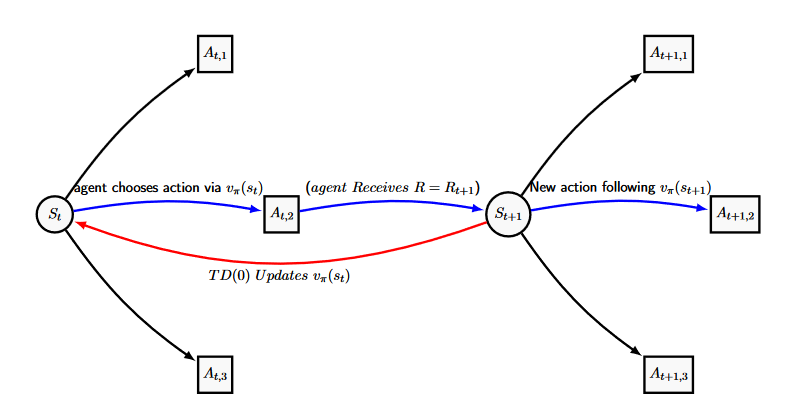
Temporal Difference learning is just trying to estimate the value function \(v_{\pi}(s_t)\), as an estimate of how much the agent wants to be in certain state, which we repeatedly improve via the reward outcome and the current estimate of \(v_{\pi}(s_{t+1})\). This way, the estimate of the current state relies on the estimates of all future states, so information slowly trickles down over many runs through the chain.
Rather than estimating the state-value function, it is commonly more effective to estimate the Action-Value pair for a particular policy \(q_{\pi} (s,a)\), for \( s \in S \) and \(a \in A\), commonly referred to as Q-Values (because a certain something came first). These are typically stored in an array, each cell referring to a specific state-action Q-Value.
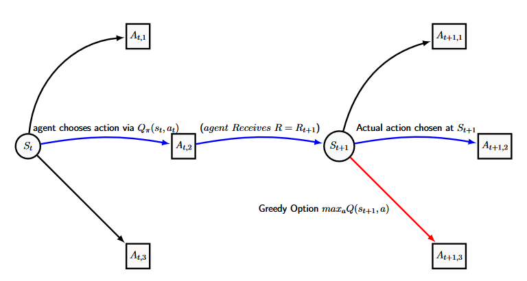
Q-Learning is arguably thee most popular Reinforcement Learning Policy method. Formally it is an Off-policy Temporal Difference Control Method, but I just want to introduce the method here. It is particularly popular as it has a formula that is both simplistic to follow and compute. The aim is to learn an estimate \(Q(s,a)\) of the optimal \(q_{*}(s,a)\) by having our agent play through and experience our series of actions and states, updating our estimates following
\begin{equation}\label{Q_Learning}
Q(s_t,a_t) \xleftarrow[]{} Q(s_t,a_t) + \alpha[r_{t+1} + \gamma max_{a} Q(s_{t+1},a) – Q(s_t,a_t)].
\end{equation}
Here our Q-Values are estimated by comparing the current Q-Value to the reward gained plus the maximal greedy option available to our agent during the next state \(s_{t+1}\) (A similar figure to the one for TD(0) is below), and hence we can calculate our estimated action-value function \(Q(s,a)\) directly. This estimate is all independent of the policy currently being followed. The policy the agent currently follows only impacts which states will be visited upon selecting our action in the new state and moving there-after. Q-learning performs updates only as a function of the seemingly optimal actions, regardless of what action will be chosen.
SARSA is an on-policy Temporal Difference control method and can be seen as a more complex Q-Learning method. By on-policy, we refer to the idea that the estimate of \(q_{\pi}(s_t,a_t)\) is dependent on our current policy \(\pi\) and we assume when we make the update that we will continue with \(\pi\) for the remainder of the agents current episode, whatever states or actions that might include them choosing. For the Sarsa Method, we make the update
\begin{equation}\label{SARSA}
Q(s_t,a_t) \xleftarrow[]{} Q(s_t,a_t) + \alpha[r_{t+1} + \gamma Q(s_{t+1},a_{t+1}) – Q(s_t,a_t)].
\end{equation}
The SARSA algorithm has one conceptual problem, in that when updating we imply we know in advance what the next action \(a_{t+1}\) is for any possible next state. This requires that we step forward and calculate the next action of our policy when updating, and therefore learning is highly dependent on the current policy the agent is following. This complicates the exploration process, and it is therefore common to use some form of \( \epsilon -soft \) policy for on-policy methods.
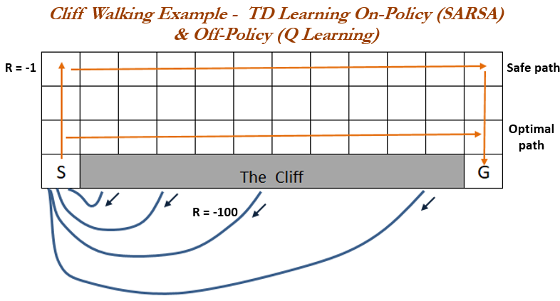
But which one is better? The cliff walking example is commonly used to compare Q-Learning and SARSA policy methods, originally found in various editions of Sutton & Barto (2018), and can be found in various other texts discussing the differences between Q-Learning and Sarsa such as Dangeti (2017) who also provides a fully working python example. Here, our agent may move in any cardinal direction at the cost of one unit, and if they fall off of the cliff they incur a cost of 100. Our aim is to find the shortest path across. The cliff example highlights the differences caused by the TD error terms between the two methods. Q-Learning could be seen as the greedy method as it always evaluates using the greedy option of the next state regardless of the current policy, and so as it walks the optimal path there exists a small random chance of choosing to fall of the cliff where the agent is punished significantly. Sarsa, however, always routes the longer yet safer path. The example shows that, over many episodes, SARSA regularly outperforms Q-Learning for this example.
So what’s the limit then? Well both of the two big-dogs of Reinforcement Learning have many improvements: Double learning to reduce bias and TD(\( \lambda \)) methods to improve convergence, but they all are limited by storing our Q-Values in some great table or array. Now this is fine for millions, even tens-of-millions of states, but there are \(10^{170} \) unique states in the ancient boardgame Go. Next time, we’ll be taking a look into combining Q-Learning with Artificial Neural Networks, and how computers finally trumped humans in the ancient boardgame Go. All the best,
– Jordan J Hood