As in many areas of statistics, big data has become an increasingly common feature of environmental data analysis. Between satellite instruments, climate models, in-situ measurements, and everything in between, huge quantities of data can be accessed from a broad range of resolutions both spatially and temporally. Using the full extent of these datasets – and in some cases combining multiple datasets in a single analysis – is often a challenge purely from a computational perspective for most moderately complex models. This is before the specific characteristics of the dataset are considered, which may themselves provide further challenges to be overcome in the modelling process.

In the context of DSNE’s work, let’s say we wanted to examine surface temperature measurements for Greenland (in the context of ice melt) by applying extreme value models. Among the many choices available – weather stations and satellite datasets being the main sources– we choose MODIS satellite data for its high spatial and temporal resolution, with around 20 years of 1km daily data available. This gives us over 7,000,000 observations in each of the nearly 7,500 days. While this is more than enough data to get a clear overview of the ice sheet, for increasingly complex models the scale of the dataset quickly becomes a challenge. For spatial extremes this is particularly true, with some models currently able to handle hundreds of points compared to the millions that would be required for an analysis of the entire dataset.

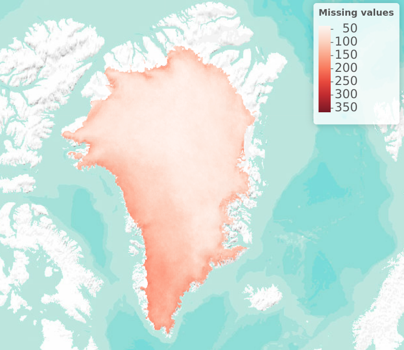
Figure 1: Number of missing days of data in each pixel in 2012, the warmest year of the past decade.

However, aside from the computational issues, statisticians and data scientists unfamiliar with satellite data may see limited problems with larger datasets. Whereas in-situ sensors can fail and sometimes take weeks to repair due to their remote locations, satellites are in constant orbit around the earth and therefore, in theory, should avoid issues relating to missing data. It’s only when you begin to visualise the data that this assumption breaks down and the extent of missing data can be seen. Because surface temperature is measured by the satellite using infrared frequency measurements, any clouds between the surface and the satellite at the time of measurement can interfere with the value measured and are therefore filtered out of the dataset. This leaves large areas of the ice sheet with missing data and means that no single day has complete coverage for the entire ice sheet. Also, since cloudy days are on average warmer than clear days, many of the warmest temperatures are missing from the dataset, which is particularly troublesome in the case of extreme value analysis that focuses on the warmest observed temperatures.

Even with the added caveat of conclusions only being valid for clear sky days, the size of the dataset also masks smaller-scale properties of the dataset that require consideration. Although not visible when plotted for the entire ice sheet, the effective resolution of the data is slightly lower than the number of points would suggest due to repeated values in neighbouring spatial points. When plotted at a fine scale, the data has series of points that have identical values throughout the time range of the dataset. Again, this creates further challenges from a modelling perspective. Fitting independent extreme value models to each point results in many points that have identical parameters, while spatial models that analyse the range of dependence between extreme temperatures at different points will be highly influenced by series of identical values that affect the estimated range of dependence between points.

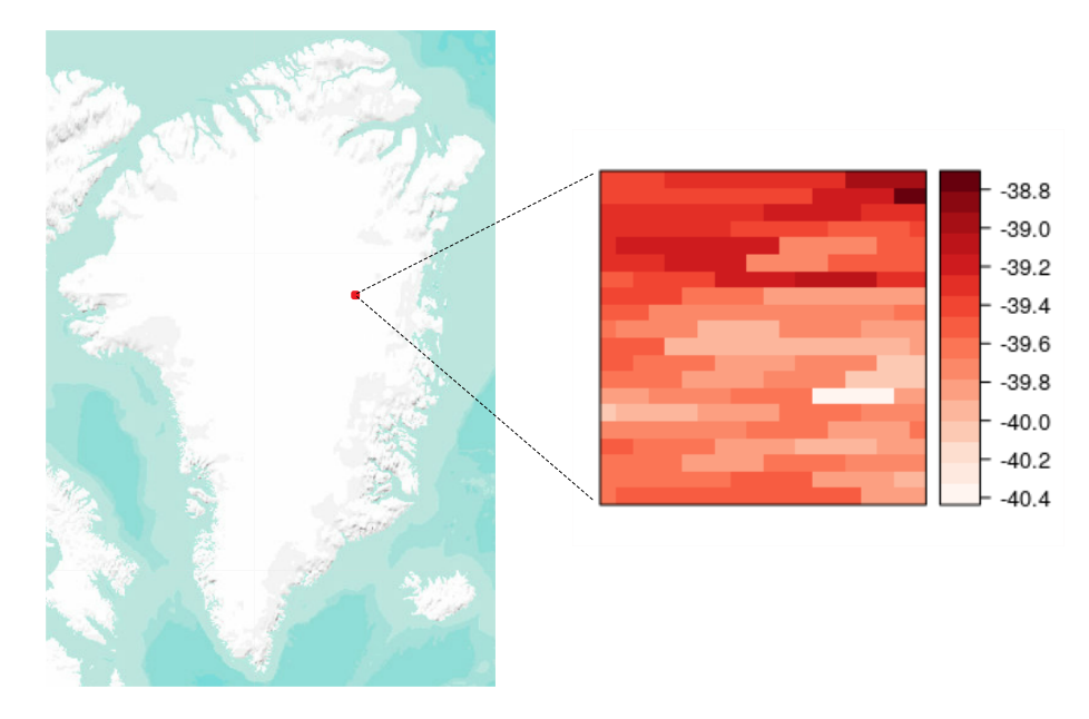
Figure 2: MODIS temperature values for 01/01/12 for a subset of the ice sheet.

The properties of the data have a huge impact on the modelling techniques used, particularly in the case of extreme value modelling of temperature data. As the scale and spatial coverage of the dataset increase, it can be easy to overlook some of the finer details of the data and make assumptions based on our expectations of the data source. Methods such as subsampling, truncated distributions, and data aggregation have all been used in our work solely due to the characteristics of the dataset to maintain confidence in the analysis that is produced. Before we begin to consider the computational cost of our analysis, it is crucial that we fully understand the features of the dataset we’re working with, even if those features are buried in resolution and hidden from an initial exploratory analysis.

Related Blogs

• 

  Annual meeting of the Society for Decision Making under Deep Uncertainty, 2022

• 

  The Cryosphere 2022 Conference

• 

  DSNE Reseachers receive best poster award at CDE Conference 2022

Disclaimer

The opinions expressed by our bloggers and those providing comments are personal, and may not necessarily reflect the opinions of Lancaster University. Responsibility for the accuracy of any of the information contained within blog posts belongs to the blogger.